
REGIONAL ECONOMIC CONVERGENCE IN THE EURO AREA
Francesco G. TRUGLIA  *
*
Alessandro ZELI *
Abstract. The study of the convergence of the euro area (EA) regions allows to test theoretical hypotheses such as: the ex-post satisfaction of the OCA conditions and the resilience to the crisis of the OCA countries. Related to these facts, it has to be noted the emergence of new centers and peripheries in the European Union and euro area. We considered the per capita GDP over the period 2001–2018, the analysis is carried out by applying different methodologies such as: convergence indicators and spatial statistics models. Our results confirm the presence of divergent processes among the EA regions.
Key words: optimal currency area, euro area, regional convergence, beta-convergence, center, periphery.
1. INTRODUCTION
During the 1990s, the European economic landscape underwent a profound transformation. Major European countries transitioned from the European Monetary System to the euro, centralising monetary policy under the control of the European Central Bank. Another key shift was the expansion of the European Union (EU) eastward, incorporating ten additional countries from Eastern and Southeastern Europe. The introduction of the euro carried an implicit promise: extending economic prosperity from the more developed Northern European countries (the EU core) to the less developed nations of Southern and Eastern Europe (the EU periphery). Many economists, therefore, anticipated a convergence process, expecting all economies to gradually align with Northern Europe’s higher standards (see De Grauwe and Mongelli [2005] for a literature review on this topic).
In the second half of the 20th century, with the creation of a single market for goods, and through the early years of the 21st century, economic growth convergence (or at least the achievement of a common growth rate) was largely accomplished. The introduction of fixed exchange rates in the mid-1990s and the adoption of the euro in 1999 further advanced this convergence process by unifying and liberalising financial markets while eliminating exchange rate risks. However, new divergence patterns emerged, particularly in terms of per capita income. These divergences can be classified along a core-periphery axis (Gräbner and Hafele, 2020; Regan, 2017). The adoption of the euro redefined the economic landscape, reinforcing a new core in Northern Europe while establishing new peripheries in Southern and Eastern Europe. These new divisions overlapped with pre-existing national disparities, sometimes blurring them, but in other cases, amplifying them. Although these trends began taking shape in the late 1990s, they became fully evident following the 2008 subprime and sovereign debt crises.
In the aftermath of the 2008 crisis, it became possible to distinguish between different groups of countries. The first group includes eurozone countries and other EU members outside the euro area. The second group differentiates between core and peripheral countries within the eurozone (Regan, 2017). According to Monfort (2020, p. 6), this issue has two dimensions: a reduction in regional disparities within the EU-28 (at least until the 2008 crisis) and a subsequent stagnation or even reversal of the convergence process. These trends appear to be primarily driven by developments in the EU core, best represented by EU-15 statistics. Unlike the broader EU, the EU-15 countries experienced stagnant divergence indicators until 2008, followed by a sharp increase. Given the economic weight of EU-15 countries, this increase significantly contributed to the overall rise in regional divergence across the EU-28 between 2009 and 2018. Notably, the EU-15 largely overlaps with the euro area, with key exceptions such as the United Kingdom and Sweden. The difference between the EU-15 and the EU-28 primarily lies in the inclusion of newer Eastern European Member States.
The data highlight a dual polarisation. On the one hand, there has been significant convergence among EU regions, primarily driven by Eastern European countries and non-eurozone members. On the other, divergence has increased among eurozone regions (Caraveli, 2017; Franks et al., 2018). At the national level, this polarisation manifested itself as reduced disparities within Northern eurozone countries (the EA core) while simultaneously pulling down the most advanced regions in Southern eurozone countries (the EA periphery) toward lower convergence levels (Monfort, 2020, p. 18).
This study aims to examine the emergence of European regional clusters, as described by Gräbner and Hafele (2020), and to identify the key drivers behind divergence trends among these regional subsets. Given that regional convergence at the European level also has implications for national convergence, we further explore intra-country convergence and divergence patterns. Our analysis focuses on the first two decades of the 21st century (2000–2018), a period marked by the introduction of the euro and the double financial crises (subprime and sovereign debt crises).
Our main objective is to determine whether a divergence process is underway among eurozone regions and between EA and non-EA countries. Additionally, we assess whether this divergence is linked to the double-dip crisis, whether national borders play a role in shaping these trends, and whether the gap between the richest and poorest regions has widened or narrowed. In this way we test the presence of endogenous OCA properties, i.e. if the a priori Oca conditions can be fulfilled ex-post.
To analyse the EU’s regional convergence process, we focus on eurozone countries to assess the impact of the crisis on the EA and the resilience of the euro system in terms of regional convergence and balanced territorial growth. Our findings indicate evidence of convergence among EA regions during the first decade following the introduction of the euro, with Northern regions (the core) experiencing upward convergence, while other (peripheral) regions exhibited divergence after the 2008 crisis. We identify convergent and divergent regional clusters and analyse their geographical distribution. Furthermore, we investigate whether this pattern is widespread across peripheries and explore the new and pre-existing dynamics shaping these countries’ trajectories.
A range of methodologies is employed in this regional analysis, including convergence indicators and statistical spatial models. Specifically, we apply spatial-lag models within the framework of the β-convergence approach.
The paper is structured as follows: Section 2 provides a theoretical overview; Section 3 describes the data and variables; Section 4 outlines the methodology; Section 5 presents the findings; Section 6 discusses the results; and Section 7 concludes. Statistical tests are included in the Appendix.
2. THEORETICAL OVERVIEW
2.1. Country-level convergence
Mundell (1961) was the first to explore the economic conditions for an optimal currency area (OCA), arguing that countries aiming for a common currency should have fully mobile factors of production – capital and labor – across borders. His primary focus was on labour mobility, assuming that capital was inherently mobile. Subsequent refinements to Mundell’s theory by McKinnon (1963) and Kenen (1969) highlighted additional necessary conditions, including commercial openness, diversification of production and consumption structures, and fiscal transfers. These conditions are essential not only for the establishment of a monetary union but also for its long-term survival. By ensuring a more symmetrical distribution of economic shocks, they help mitigate the costs associated with losing independent monetary policy and exchange rate flexibility.
McKinnon (1963) emphasised two key factors for the success of a single currency area. First, labour mobility between less developed and more developed regions within the currency union is crucial for balancing initial economic disparities. Second, enhancing internal mobility across industries helps counteract technological disadvantages among different regions within the union.
While these conditions primarily focus on short-term economic convergence, this study examines GDP per capita (in levels) due to its established link with business cycle synchronization among EA countries. Numerous studies suggest that economic divergence (in levels) correlates with the lack of synchronisation in business cycles. Koren and Tenreyro (2007) and Beck (2013) demonstrated that GDP per capita convergence is associated with greater business cycle synchronisation. Specifically, Koren and Tenreyro (2007) identified technological diversification – firms or sectors utilising a wide variety of inputs and advanced skills – as a key factor in reducing business cycle volatility.
Recent studies have extensively analysed business cycle synchronisation and GDP growth within the euro area, the most significant single currency area today. Two notable surveys are de Haan et al. (2008) and Stoforos et al. (2024). De Haan et al. (2008) reviewed multiple empirical studies and found that while euro area business cycles became more aligned after the 1990s, “the business cycles of many euro countries are still substantially out of sync” (Haan et al., 2008, p. 266). Stoforos et al. (2024) presented similarly mixed results, particularly due to the impact of the 2008–2011 double-dip crisis. Their survey highlights two key trends. First, they identify two distinct periods: from the 1990s until the crisis, a process of convergence was underway; after the crisis, peripheral countries began to diverge. As they note, “until 2007, business cycle synchronisation favoured the operation of a single currency, but the recession and the subsequent Eurozone crisis led to desynchronisation, particularly for periphery countries like Greece” (Stoforos et al., 2024, p. 229).
The second trend observed is increasing business cycle synchronisation among Eastern European countries that joined the EU after 2000. Several studies report a rising convergence in business cycles for these countries, as well as for the Balkans.
When the euro was introduced between 1999 and 2002, not all EA countries met the conditions outlined by Mundell, McKinnon, and Kenen. However, some researchers, such as Frankel and Rose (1997) and Rose (2000), argued that the OCA theory had endogenous properties: simply creating a currency union would trigger a convergence process, enabling the initial conditions to be fulfilled ex post. This led to two competing perspectives in academic debate.
The first perspective, known as the European Commission view (European Economy, 1990), asserts that as EA countries reached a certain level of economic integration, the likelihood, frequency, and intensity of asymmetric shocks would decline. The second, known as the Krugman view (Krugman, 1993), identifies four economic consequences of integration: regional specialisation, instability of regional exports, pro-cyclical capital flows, and divergence in long-run growth.
According to the first view, convergence should have been driven by capital and labour mobility. Lower labour costs in less developed peripheral regions, combined with the equalisation of interest rates, were expected to attract investment to these areas (De Grauwe and Mongelli, 2005). Neoclassical theories (Blanchard and Giavazzi, 2002) suggest that removing obstacles such as exchange rate risk and capital flow restrictions should increase capital inflows to peripheral economies while encouraging labour migration from lower-wage to higher-wage countries, equalising the marginal product of labour. Consequently, in the early years of the euro, there was a prevailing belief that the endogeneity of the OCA paradigm would ultimately prevail.
Although per capita income convergence is not a strict prerequisite for an OCA to function, it is a key objective in any economic integration process (Franks et al., 2018). As previously discussed, long-run growth and short-term economic fluctuations are interconnected. A gradual reduction in income disparities across countries and regions facilitates wealth-sharing among areas with different growth rates. Moreover, income convergence fosters a more favourable public attitude toward common financial instruments by reducing concerns about establishing a permanent transfer mechanism between core and peripheral regions (IMF, 2008).
Other factors, such as diminishing economies of scale and weakening agglomeration effects (e.g., due to the increasing dominance of the service sector), were also expected to reduce economic asymmetries across countries and regions (De Grauwe and Mongelli, 2005). Another crucial OCA property is resilience to external shocks. Countries in a monetary union should experience fewer asymmetric shocks, as economic structures become more similar over time. As a result, a single monetary policy should suffice for all members. The key conditions to minimise asymmetric shocks include similarity in economic structures, high intraregional trade, low specialisation, homogeneity of preferences, mobility of production factors, and the presence of transfer payments (Hafner and Jager, 2013).
An alternative theoretical approach focuses on varieties of capitalism (Hall, 2012; Regan, 2017). Northern EA countries rely on export-led growth, while Southern countries follow a domestic demand-led growth model. These two economic models are inherently difficult to reconcile within a single monetary area. The double-dip crisis hit Southern countries particularly hard, and the proposed solution was for all EA members to converge toward an export-led growth model. However, this approach exacerbated economic imbalances by forcing Southern countries to adopt internal devaluation policies. The result was intensified competition over real wage levels between Northern and Southern regions, deepening existing asymmetries in the euro’s structural foundations.
Thus, industrial specialisation has increased the euro area’s vulnerability to asymmetric shocks. Furthermore, given the lack of compensatory mechanisms – such as labour mobility and transfer payments – the euro area has struggled to respond to crises in a balanced manner that benefits all member states (Hafner and Jager, 2013).
2.2. Regional convergence
Regions within EA countries can be viewed as regions within a nation undergoing unification (the EA itself). However, the process of regional economic convergence within nations follows different dynamics than convergence between nations. Political unification presents both advantages and challenges for regional convergence.
On the one hand, regional convergence can be facilitated by removing external constraints and creating conditions for rapid capital accumulation. A newly unified entity can implement standardised tax and social security systems that help equalise per capita income. In this sense, if production factors are mobile, regional convergence may be easier to achieve than convergence between independent nations.
On the other, economic activity tends to concentrate in established economic centres, potentially hindering the rapid convergence of peripheral areas. Scale economies and the attractiveness of industrial clusters or urban hubs (agglomeration economies) may reinforce the economic dominance of the wealthiest and most central regions. Additionally, financial transfers from central governments to less developed regions could create long-term dependence, rather than fostering sustainable growth. If wages are equalised across regions despite differences in productivity, peripheral areas may lose competitiveness, discouraging capital inflows and encouraging capital outflows toward the economic core.
A recent survey (Stoforos et al., 2024) highlights the need for further research on regional convergence and business cycle synchronisation, as most studies focus on national-level dynamics. This survey confirms the presence of a national border effect, meaning that regions within the same country tend to be more synchronized than those in different countries. Many empirical studies reviewed in this paper report no significant regional convergence and a persistent influence of national business cycles on regional development. Furthermore, socio-economic and structural factors play a crucial role in regional economic performance, with spillover effects between neighbouring regions. For example, high-income clusters in Western Europe have positively impacted adjacent areas.
Previous research suggests that regional convergence within the EU, and particularly within the EA, has followed a nonlinear trajectory: initial convergence was followed by stagnation and, in some cases, divergence (Díaz del Hoyo et al., 2017; Diermeier et al., 2018; Monfort, 2020). Specifically, income convergence remained stable during the early years of the euro’s introduction, but after the financial crisis, the trend reversed toward increasing divergence (Franks et al., 2018).
While Eastern European countries have consistently experienced convergence, Italy, Greece, and the United Kingdom have undergone divergence. As a result, the convergence process that had been ongoing within the EU-15 since the 1950s came to an end before 2012 (Goecke and Hüther, 2016). In Greece, Ireland, Portugal, Spain, and Italy, convergence turned into divergence, although recent trends suggest a possible reversal for Spain, Portugal, and Ireland (Goecke and Hüther, 2016).
A recent study by Diemer et al. (2022) examined regional growth patterns within the EU, applying the development trap theory, which affects middle-income regions in several European countries. The authors incorporated productivity and employment measures alongside per capita income ratios. However, the regional classifications in their study align closely with those found in this paper. We argue that a deeper explanation of these trends lies in economic policy decisions, particularly the introduction of the euro and the absence of effective convergence policies.
On the subject of intra-country regional differences, EA countries have different paths of convergence. In Italy, the pace of gap development between the southern industry and the centre-northern industry has increased in recent years because of a strong and rapid increase in competitive pressure due to European integration in the production system. Conversely, on the other hand, the more industrialised areas of the northwest had difficulty catching up, as they lagged behind in growth compared with other most industrialised European regions. In Germany, evidence (Weddige-Haafa and Kool, 2017) showed a faster convergence of the West and East regions in 2005–2014 compared with the previous period (1995–2005), signalling an income divergence between West German states. The EU accession of Spain in the 1980 s resulted in a strengthening of regional convergence processes and a decrease in interregional disparities (Wójcik, 2017). However, until now, strong income and productivity gaps remain between the core regions (Madrid, Navarra, Catalunya, and Basque region) and the peripheral regions (Extremadura, Andalusia, Castilla-La-Mancha, and Galizia). Moreover, France has shown evidence of divergent trends between the peripheral regions and the core (Ile de France) (Alcidi et al., 2018b).
3. DATA AND VARIABLES
A more detailed regional-level analysis is useful to complement country-level studies, particularly in assessing the effectiveness of a common monetary policy and evaluating whether the European Commission view or the Krugman view better explains economic dynamics. In this paper, we analyse regional divergences in gross domestic product (GDP) per capita, a key indicator of economic growth that allows for meaningful territorial comparisons. The analysis is based on OECD data and follows the Eurostat Nomenclature of Territorial Units for Statistics (NUTS), the standard classification for regional data in European countries. The EU divides its member states into three NUTS levels according to administrative structure: NUTS1: Broad regional aggregations, such as German federal states. NUTS2: Intermediate regional units, such as Spanish autonomous regions and French or Italian regions. NUTS3: The smallest subregional areas.
This study uses NUTS2 regions as the statistical units of analysis. The variable under investigation is regional income per capita, calculated as the ratio between regional GDP and regional population. Changes in GDP per capita serve as a reliable proxy for economic growth trends. The data, expressed in euros at constant prices, cover the period 2001–2018, ensuring comparability across all EU and EA countries.
The analysis includes the following EA countries: Germany, France, Italy, Spain, Portugal, Belgium, the Netherlands, Luxembourg, Austria, Finland, Estonia, Latvia, Lithuania, Slovakia, Slovenia, Greece, Malta, and Ireland. Additionally, we examine the non-EA EU countries: Hungary, Poland, Bulgaria, Romania, the Czech Republic, Denmark, the United Kingdom, and Croatia.
A total of 202 territorial units (regions) are analysed: 130 regions within EA countries; 72 regions in non-EA EU countries. Although some countries joined the EA after 2002, we classify all countries that were part of the EA in 2018 as EA members throughout the analysis. This approach minimises bias, as economic convergence processes typically begin a few years before formal EA accession. For Ireland and Lithuania, we consider the entire country rather than NUTS2 regions for practical reasons.
4. METHODOLOGY
In our analysis we apply, differently from other studies (Esteban, 2000; Díaz Dapena et al., 2019), as methodological instrument statistical spatial models and also convergence indicators. In the following section, we describe the methodological features of both statistical approaches.
4.1. Divergence indicators
The regional divergence of the GDP per capita is analysed by explaining two divergence indicators: the Williamson index and the Theil index, which have been used in similar studies (Malanima and Daniele, 2007). The Williamson index can be calculated as follows:
(1)
Where yi is the GDP per capita in the i-th region, ym is the average GDP per capita, and p is the population with the same notation. The Theil index, calculated at time t, is expressed as follows:
(2)
where xi = yi/yT is the GDP share of region i, and qi=pi/pT is the share of the population. We consider all regions in the EU, but the indexes are calculated separately for the regions in the EA and for the countries outside of it.
4.2. Beta convergence
Among the different procedures used for territorial convergence analysis, for which a broad litature exists (Taufer et al., 2016), we use the β-convergence approach in this study. In this approach, changes in territorial divergences relative to a specific variable are registered over a certain period. If the changes in territorial divergences decrease, a convergence process takes place, and the convergence parameter b1 takes a negative sign. The basic model can be written as follows:
vi = β0 + β1 lny0, i + εi
(3)
where yi = ln(vt /v0)/T is the natural logarithm of the average change over time T, and εi is the stochastic component. Therefore, the β-convergence model registers the convergence speed and is a function of the parameter β1 (Arbia 2014).
β1 = –(1 – e–bt)
which produces
The valuation of the longitudinal economic effects of the EA should also consider the spillover effects on territorial units. For this purpose, considering some results of the preliminary analysis, a spatial – lag model is used to spatially regress the dependent variable. A dummy variable to discriminate the divergent and convergent regions in the EA for the period of 2008–2018 is also considered. The model, including a spatial lag, is expressed in the following matrix format (Cliff and Ord, 1981; Anselin, 1988):
y = ρW1y + Xβ +ε with |ρ| <1
(4)
ε = λW2 ε + u with |λ| <1
(5)
where y is vector N x 1 of the observations of the dependent variable (N is the number of geographical units), W1 and W2 are matrixes of continuity N x N associated with the lag and error variables, and X is a matrix N x k of observations of the explanatory variables. Measures ρ and λ are the two (scalar) autoregressive coefficients associated respectively with lag variable y and error factor ε, while β is the k x 1 vector of the parameters associated with the explanatory variables X. Finally, u is the error term, which shows normal distribution with 0 mean and diagonal covariance matrix Ω.
Since there are three autoregressive terms in the general model (ρW1y e λW2 ε), the ordinary least squares (OLS) method of estimation produces inaccurate estimates with little consistency, thereby proving biased estimates. Consequently, the maximum likelihood method (ML) is applied; in this case if:
– ρ and λ = 0 we obtain the classical regression model
y = Xβ + ε;
(6)
– ρ = 0 we obtain the error model
y = Xβ + (I – λW2)–1u
(7)
– λ are set at 0, we obtain the lag model.
y = ρW1y + Xβ + ε
(8)
The concept of spatial dependence assumes different meanings according to the applied model (Doreian, 1980). The ρ parameter of the Spatial lag model represents the relationship among the territorial units in terms of the dependent variable.
The parameter λ of the Spatial error model represents the combined effect due both to the spatial configuration of the variables and the variables not included in the model. The statistics for model identification (Appendix A, Table A.3) suggested the presence of spatial lag for the dependent variable. Finally, we estimated the following β-convergence model:
tgpi,t = ρWtgpi,t + α + βgpi,t–1 + ϵi
(9)
Where:
– tgpi,t is the natural logarithm of the per capita GDP growth rate;
– Wtgpi,t represents the spatial lag for the dependent variable: in other words, the regional growth rate also depends on the growth of neighbouring regions;
– gpi,t–1 = ln(vi, t–1) is the natural logarithm of the initial per capita GDP;
– β is the parameter that signals the presence (if negative)/ absence (if positive) of convergence;
– ρ is the spatial autoregression parameter;
– εt, i ~ N(0, σ2) represents the error.
5. RESULTS: REGIONAL DIFFERENTIAL GEOGRAPHY IN THE EA
5.1. Introduction
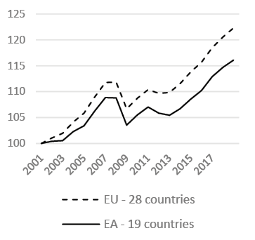
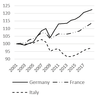
We first consider the framework that includes the trends and dynamics from our analysis. We present the GDP per capita trends in the EU and EA, which are divided into e three main countries in the EA (Fig. 1).
Source: own work based on OECD data.
Source: own work based on OECD data.
The EU GDP per capita trend shows an increasing trend before and after the double-dip crisis, even at a slower pace in the second period. The EA countries register an even slower pace compared with the EU as a whole (Fig. 1a). If we examine the GDP per capita trend of the main economies in the EA (i.e., Germany, France, and Italy), the growing pace of Germany accelerates after the crises and overcomes the results of the other two countries (Fig. 1b). This is a sign of an ever-deeper divergence among the different zones in the EA.
5.2. Geography of divergence
The descriptive analysis takes into account the GDP per capita differentials compared with the EA average at three specific points in time: the 2001 (introduction of the euro), 2007 (the year before the subprime crisis), and 2018 (last available year before the COVID-19 global pandemic). The regional differentials are calculated as the GDP per capita percentage differences with respect to the EA average.
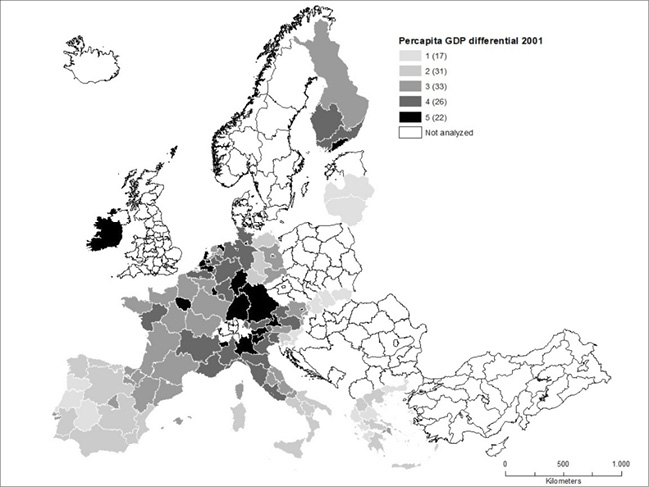
Note: 1: < 50%; 2: 50%–75%; 3: 75%–100%; 4: 100%–125%; 5: >125%. EA borders in 2018 (Germany, France, Italy, Spain, Portugal, Belgium, the Netherlands, Luxembourg, Austria, Finland, Latvia, Lithuania, Slovakia, Slovenia, Greece, Malta, and Ireland). Euro constant values.
Source: own work based on OECD data.
The regional differentials map for year 2001 (Fig. 2) registers a more developed central area that has Germany as a pivot. Next to this central area is an Alpine–Mediterranean zone extending from the Alps to the Po Valley to the south and the Netherlands and the North Sea to the north. The regions, including the capitals, highlight the major GDP per capita values. Therefore, Ile de France, Madrid, Helsinki, the Attic, Latium, Hamburg, Berlin, Lisbon, Holland, and Vienna present greater values than the adjacent regions.
The most underdeveloped regions are located in the south (Southern Spain, the Italian Mezzogiorno, and Greece) and in the east (Baltic countries, East Germany, and Slovakia). Compared with the map for 2001, the map for 2007 registers upward and downward movements. The latter is mainly due to a decline in some Italian and French regions (Fig. 3).
Specifically, Lombardy in Italy and some regions in the French West (Pays de la Loire) show a decrease in GDP per capita values compared with the EA average.
Greece, as a whole, lags significantly behind. The regions of the Iberian Peninsula increase their ranks. The regions registering an increase in GDP per capita are located in Finland and Austria.
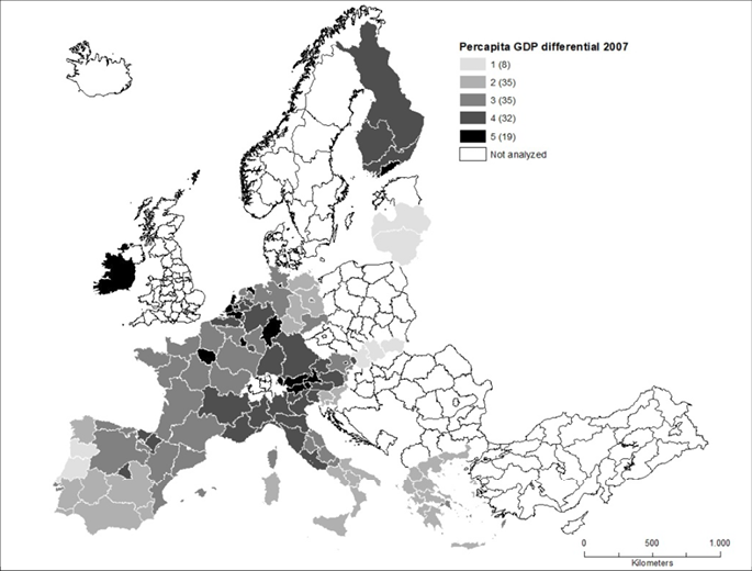
Note: 1: <50%; 2: 50%–75%; 3: 75%–100%; 4: 100%–125%; 5: > 125%. EA borders in 2018 (Germany, France, Italy, Spain, Portugal, Belgium, Netherlands, Luxembourg, Austria, Finland, Latvia, Lithuania, Slovakia, Slovenia, Greece, Malta, and Ireland). Euro constant values.
Source: own work based on OECD data.
In 2018, 10 years after the subprime crisis and seven years after the sovereign debt crisis, the regional divergences within the EA notably increased. As shown in Figure 4, in terms of the GDP per capita, the northern regions rank high in the EA, whereas the southern regions rank low. For the Italian and French regions, divergence is significantly augmented. In Italy, the central geographical macro-region loses position, specifically Latium and Umbria. In France, the macro-regions of Rhone-Alpes and Auvergne, located in the centre of the country, lag behind in terms of the GDP.
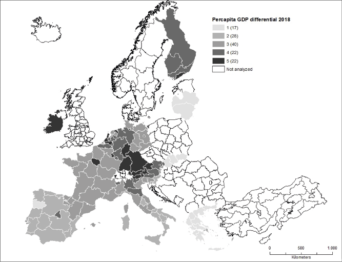
Note: 1: < 50%; 2: 50%–75%; 3: 75%–100%; 4: 100%–125%; 5: > 125%. EA borders in 2018 (Germany, France, Italy, Spain, Portugal, Belgium, Netherlands, Luxembourg, Austria, Finland, Latvia, Lithuania, Slovakia, Slovenia, Greece, Malta, and Ireland). Euro constant values.
Source: own work based on OECD data.
The changes are concentrated in these regions, and the rest remain unchanged. The Iberic peninsula and Greek regions generally rank last. The regions of the Italian Mezzogiorno do not register any change in pace in catching up with the North European regions, similar to the Greek and Eastern regions. This means that the GDP per capita increments registered in the post-crisis period for the EA were not uniformly shared among the different economic areas within the EA and that some regions had more advantages than others, as shown by the main countries in Figure 1b.
In terms of the different paths followed by the regions with capital cities, these regions generally outperform the other regions in a country (Alcidi et al., 2018a), especially when the role of the capital city is coupled with the role of the financial centre. The regions with capital cities and financial centres perform better than others, even if a general lag-down is registered in the rest of the country, as in France. Therefore, the continental financial centres, such as Frankfurt, Paris, Luxembourg, and, also, Dublin, outperform (Gräbner and Hafele, 2020) other regions, even if there is a general lagging back, as in France. This is another factor increasing divergence among regions (Degl’Innocenti et al., 2017). In countries where the crisis strongly hit and where were not present financial centres, as in Italy and Greece, the regions seats of capital cities notwithstanding perform better than the other regions, however lose positions.
5.3. Divergence indicators
Figure 5 shows the Williamson (W) and Theil (T) indices calculated for the EA and for most non-Euro countries in the EU in 2001–2018.
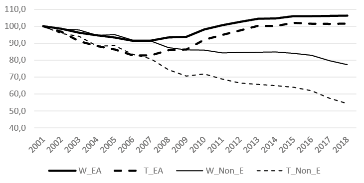
Note: Index number calculated for the W and T indices and based on 2001. EA borders in 2018 (Germany, France, Italy, Spain, Portugal, Belgium, Netherlands, Luxembourg, Austria, Finland, Latvia, Lithuania, Slovakia, Slovenia, Greece, Malta, and Ireland). The non-Euro EU countries considered here are Hungary, Poland, Bulgaria, Romania, Czech Republic, Denmark, Sweden, the United Kingdom, and Croatia. US dollar constant values.
Source: own work based on OECD data.
The Williamson and Theil indices present the same trends in the two country groups. The regional divergence indicators for the EA countries as a whole show a strong time-dependent path. A convergence of the GDP per capita is observed in the first period of 2001–2007; the same result is observed for the non-Euro regions in the same period. Starting in 2008, the differences among the EA regions increase to offset, or more than offset (in the case of W_EA), the gains in terms of convergence achieved in the first period. The trend of the indicators makes it possible to identify two well-defined periods for the EA regions. In the first period (2001–2007), the introduction of the euro caused a slight convergent push among the EA regions. This is probably due to capital inflows and the creation of financial bubbles caused by the downward convergence of interest rates and the contemporaneous maintenance of inflation differentials between the core and peripheral countries. The first-period convergence seems to depend on the convergence of some northern regions (Finland and East Germany) toward the average levels rather than on sustained growth by the peripheral regions. After the subprime crisis and the sovereign debt crisis (2008–2018), the capital inflow reversal and the launch of pro-cyclical economic policies, which mainly hit the peripheral regions, determined an increase in divergence processes among the EA regions. Note that the EU regions outside the EA continued their convergence path, which seemed unaffected by the double-dip crisis, and thus did not present the same time path as the EA. This shows a strong sign of how an economic crisis (in a monetary union) is an important factor in generating imbalances among regions and countries.
5.4. Regression results
As described in Section 4, we estimate an econometric model for each sub-period (2001–2007 and 2008–2018) using the β-convergence approach. All variables are taken in the logarithms.
5.4.1. First period (2001–2007)
We first estimated the OLS model (Equation 3) and performed statistical tests to verify whether the data were better fitted by a spatial error model or a spatial–lag model. A spatial–lag model was then estimated. The OLS outcomes and the general diagnostics are presented in Appendix A.
Tables A.1 and A.2 show the results and statistical tests for the OLS. Table A.3 presents the diagnostics for spatial dependence. The statistical tests indicate how the spatial – lag model better fits the data: the Lagrange multiplier (lag) is greater than the Lagrange multiplier (error). On the basis of the outcomes of the diagnostics for spatial dependence, we estimated the spatial – lag model described in Equations 4 and 5. Table A.4 presents the log-likelihood ratio test comparing the OLS and spatial–lag models. As the test was significant, the second model was confirmed to be better than the first. The spatial–lag model estimates (Equation 9) are presented in Table 1.
| Variable | Coefficient | Std. Error | z-value | Probability |
|---|---|---|---|---|
| Constant | 0.118551 | 0.019014 | 6.23499 | 0.00000 |
| gp – 2001 | −0.010853 | 0.001841 | −5.89594 | 0.00000 |
| Wtgp – 07_01 | 0.530334 | 0.060527 | 8.76194 | 0.00000 |
Dep = tgp2007/2001.
Source: own work based on OECD data.
The results presented in Table 1 confirm the presence of a convergence process in the EA for the period of 2001–2007. Therefore, b1 (GDPpc_2001) presents a negative sign. Although statistically highly significant, the convergence is not very strong in terms of intensity. The highly significant and positive coefficient of the spatial dependence variable (W_LNGDP07_01) indicates a strong spillover effect on the regions. That is, the regions tend to move grouped into blocks.
5.4.2. Second period (2008–2018)
We carried out the same procedure for the second period. Table A.5 presents the results of the OLS model. In this case, the b1 coefficient is not statistically significant. The diagnostic tests (Tables A.6 and A.7) suggest the application of the spatial–lag model.
Table A.8 presents the log-likelihood ratio test comparing the OLS and spatial–lag models. The log-likelihood ratio test indicates spatial–lag as the better fitting model. Table 2 presents the spatial–lag model estimates (Equation 9).
| Variable | Coefficient | Std. Error | z-value | Probability |
|---|---|---|---|---|
| CONSTANT | −0.010115 | 0.018597 | −0.54393 | 0.58649 |
| gp 2 – 2008 | 0.000974 | 0.001820 | 0.53497 | 0.59267 |
| Wtgp – 18_08 | 0.696366 | 0.060985 | 11.4187 | 0.00000 |
Dep = tgp2018/2008
Source: own work based on OECD data.
For the spatial model calculated over the second period, we did not find a b1 significant coefficient. In other words, in the second period, there is no convergence (or divergence) process in the EA as a whole. Thus, we conducted an in-depth analysis for the second period to separately analyse the most dynamic and the most lagged back regions. Considering the preliminary descriptive analyses, we grouped the EA regions into two: the core (i.e., regions with a higher GDP per capita located in the northern countries) and the periphery (i.e., regions with a lower GDP per capita that lagged behind after the double-dip crisis and located in the southern countries).
We determined whether the convergence or divergence process occurred in these two groups. A convergence process for the core regions and a divergence process for the peripheral regions are expected. The richest regions in the north maintain (or ameliorate) their GDP per capita levels, thus maintaining their relative distances. Conversely, the peripheral regions, although lagging behind, cover different paths of divergence. The interaction of these effects yields at the aggregate level a non-significance in convergence parameter b1 , this because of the compensations due to the offsetting of the pressure to convergence and divergence coming from the different areas.
Source: own work based on OECD data.
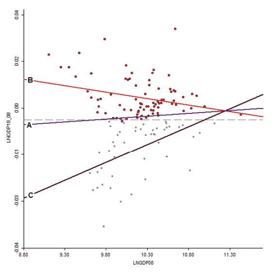
To verify these hypotheses, we defined two groups of regions, namely, the best and worst performing, over the period of 2008–2018. We calculated the regression lines that fit the coordinates (changes – initial values) for each single region. The regression lines are presented in Fig. 6 (line a), along with the regional coordinates. The best and worst results were identified based on whether the GDP per capita growth was above or below the regression line (darkest and shaded point s).
Based on this partition, we calculated two other regression lines: one for the best performers b line (core) and another for those lagging behind c line (periphery). Note that the best performers present a strong convergence tendency, whereas those lagging behind have a divergence tendency. This is confirmed by the regression outcomes presented in Table 3.
| no data | N | R2 | St. Er. (b0) | T (b0) | p-value (b0) | b1 | St. E. (b1) | T (b1) | p-value (b1) |
|---|---|---|---|---|---|---|---|---|---|
| Total | 130 | 0.005 | 0.026 | −0.726 | 0.469 | 0.002 | 0.003 | 0.769 | 0.444 |
| Group 1 (core) | 73 | 0.124 | 0.017 | 3.655 | 0.000 | −0.005 | 0.002 | −3.165 | 0.002 |
| Group 2 (periphery) | 57 | 0.180 | 0.031 | −3.748 | 0.000 | 0.011 | 0.003 | 3.480 | 0.001 |
Source: own work based on OECD data.
The results for the overall regression (first row) confirmed the absence of convergence/divergence processes, and the estimated parameters and tests described an almost a flat line. Conversely, when regression analysis was conducted on the two subsets identified before, we observed a strong convergence for the core (second row) and an even stronger divergence for the periphery (third row). Convergence speed was low in the first period (−0.00157), and no convergence was observed in the second period.
Figure 7 presents the converging and diverging regions as identified above. The converging regions are aggregated at the centre of Europe (core), while the diverging regions comprise the peripheral countries.
The regions tend to move grouped into blocks and concentrated in specific countries. Therefore, the same countries are defined as core countries or lagging-behind countries as a whole. The analysis of Map 4 presents some interesting points. Two great areas are identified: the core, which consists of Germany and its neighbouring countries, the Baltic countries, and Ireland, and the periphery, which includes Italy, Greece, Spain, Portugal, France, and Finland.
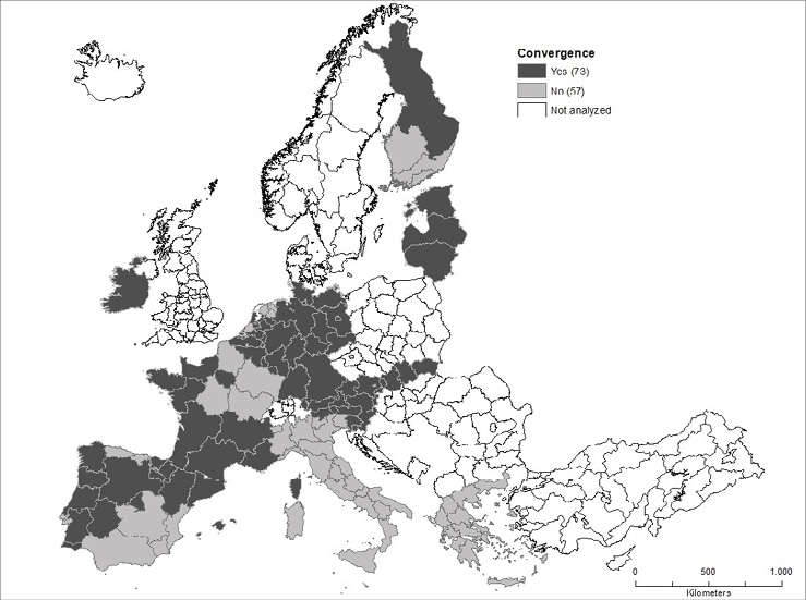
Source: own work based on OECD data.
The periphery aggregate counts countries whose regions are completely included in the lagged behind group such as Italy and Greece, the first burdened by the industrial and productivity crisis. The case of France seems to be analogous, and the most industrialised regions in the northeast of the country appear to lose their positions. For France and Italy, a decrease in internal divergence may be due more to a process of rapprochement of the more developed regions to the less developed regions rather than to an acceleration of the growing pace of the latter. Even if there are the same rapprochement signals from the regions in the Iberian Peninsula, they remain quite far from the core. Finland was severely hit by the crisis. The tighter the fiscal stance in the EA, the more the developed southern regions in the country seem to have taken a divergent path.
As highlighted above, financial centres seem to have more chances. Paris, Dublin, Luxembourg, and Frankfurt maintain their positions in the core group despite the fact that, in some cases, the rest of the country loses its position and lags behind compared with the more dynamic regions.
6. DISCUSSION
This paper contributes to the literature on regional convergence in the euro area by confirming the existence of significant variability in convergence patterns, which also depend on economic (asymmetric) shocks, particularly the double-dip crisis. The findings confirm the presence of two distinct phases: a relative convergence period lasting until the 2007–2008 crisis, followed by a phase of divergence. These results align with previous studies pointing to increasing divergence among EA regions (Stoforos et al., 2024; Beck, 2020; Beck and Okhrimenko, 2024). Furthermore, the analysis highlights a double polarisation, both within the EA and across the broader European Union.
Over the past two decades, regional convergence dynamics have revealed a double polarisation (Beck, 2020). The first form of polarisation is observed between two groups of economically converging countries: the new EU accession countries of Eastern Europe, the United Kingdom, Sweden, other northern non-euro countries (outer periphery), and the oldest EA member states (EU core). The second level of polarisation occurs within the EA, with a clear divide between the northern EA countries (internal core) and the southern EA countries (internal periphery) (Diermeier et al., 2018).
The study of regional convergence is also crucial in assessing the endogenous properties of an optimal currency area (OCA). Specifically, it examines whether the ex-post fulfilment of OCA conditions occurs through a natural convergence process among regional economies following the creation of the monetary union. Additionally, it evaluates whether the OCA framework strengthens resilience to external shocks, meaning that countries and regions within the monetary union should experience reduced exposure to asymmetric shocks as structural differences diminish. However, our findings indicate a divergent trajectory in GDP per capita, confirming the persistence of double polarisation and the emergence of core-periphery dynamics within the EU. More specifically, we identify a high-growth EU periphery, consisting of Eastern European countries outside the EA, and an internal EA periphery, composed, mainly, of southern EA countries.
This study primarily focuses on the second level of polarisation, that is, the divergence among EA regions. Differences in growth rates have led to alternating phases of convergence and divergence across various periods in European economic history. The analysed timeframe can be divided into two sub-periods: the first phase (2001–2007), characterised by slight convergence, and the second phase (post-2008 crisis), dominated by divergence. In the first period, capital inflows from core EA countries fuelled economic growth in peripheral countries, often creating speculative bubbles, such as the real estate booms in Spain and Ireland. However, when the crisis hit, these capital flows abruptly ceased, triggering a divergence process.
The economic crisis affected EA regions in different ways, as evidenced by GDP per capita differentials across various geographical areas. The observed national border effect, with regional economies moving in country-specific blocks, underscores the lack of a uniform convergence process. It is important to note that regional convergence within a single country is more likely to occur than regional convergence across different countries (Barro and Sala-i-Martin, 1992). This remains a key challenge for EA institutions. Another noteworthy finding is the inclusion of French regions in the peripheral category. Many French regions have exhibited economic stagnation similar to that of southern EA countries, with the exception of Île-de-France, which, as the capital and financial centre, follows a different trajectory (Gräbner and Hafele, 2020; Novac and Moroianu-Dumitrescu, 2020).
Our findings also reveal a synchronous movement among core regions, contrasting with the divergent trends within peripheral regions. Regional disparities have widened, but not in favour of the less affluent regions. Regions with lower initial GDP per capita experienced greater economic deterioration after the crisis, with no evidence of a catch-up process. These findings align with recent studies indicating the absence of convergence between core and peripheral countries, as well as between rich and poor regions (Beck and Okhrimenko, 2024).
Furthermore, these results suggest that European economic policies have primarily benefited northern countries, while a single economic policy cannot effectively address the diverse needs of all EA countries. Beck (2021) highlights a strong negative correlation between GDP per capita disparities and structural similarity, suggesting that further European integration could exacerbate structural divergence by increasing the risk of asymmetric shocks. This raises critical concerns regarding independent monetary policy within the EA.
The increasing regional divergence within the EA poses significant challenges to the effectiveness of the common monetary policy (Beck, 2020). There is no broad consensus in the literature regarding the impact of monetary integration on business cycle synchronisation. In some cases, monetary integration has been associated with reduced cycle synchronisation. One reason for this is that exchange rate fluctuations can act as a shock-absorbing mechanism. Without independent exchange rates, an asymmetric shock within a common currency area may lead to greater economic divergence (de Haan et al., 2008).
Additionally, under a fixed exchange rate regime changes – initial values where the central bank operates with a single monetary policy target – external shocks must be absorbed through adjustments in real economic variables, primarily labour costs (Zeli et al., 2022).
As emphasised by Caporale et al. (2015), the lack of an endogenous convergence process calls for a fundamental shift in the EU’s political and economic approach. Specifically, the following policy measures should be considered: better coordination of economic policies across different European regions to account for regional disparities, establishment of a fiscal transfer system to redistribute resources from high-productivity areas to low-productivity regions. These policy adjustments would help address the growing structural imbalances within the EA and ensure a more sustainable and inclusive economic framework for the future.
7. CONCLUSIONS
We analysed the potential convergence trends among EA regions from 2001 to 2018, a period marked by the introduction of the euro, the double-dip crisis of 2008, and new accessions in Eastern Europe.
Our findings allow us to reject the hypothesis of an ex-post (endogenous) fulfilment of the Optimum Currency Area (OCA) conditions, as we found no evidence of stable convergence processes among regions and countries, nor of a uniform and strengthened resilience to external shocks (such as economic crises). As a result, our outcomes align more closely with Krugman’s perspective than with that of the European Commission (Beck, 2024), as a result, these results seem to disprove the presence of endogenous properties of OCA.
Furthermore, our research confirms, in line with various studies included in the survey by Stoforos et al. (2024), that socio-economic and structural determinants play a crucial role in economic performance. These factors vary significantly across regions, reinforcing the link between economic growth and initially more developed areas.
The increasing divergence between core and peripheral regions has also been documented in other studies that analyse the issue from an international trade perspective (Caporale et al., 2015, p. 160).
Our paper contributes to the literature on regional convergence (Stoforos et al., 2024) also by applying spatial modelling to regional convergence in the EA area. However, we assess convergence using only one economic variable: GDP per capita. A natural extension of our analysis would involve breaking down GDP per capita into productivity and employment rate components, as proposed by Diemer et al. (2022). While productivity has generally declined in Europe over recent decades, this deterioration has been more pronounced in some countries than in others. Moreover, there has been no catch-up effect following the introduction of the euro. Countries with initially low productivity have experienced weaker productivity growth and an even steeper decline in recent years (Díaz del Hoyo et al., 2017; Franks et al., 2018). A regional-level analysis of the convergence dynamics in terms of productivity and employment rates among EA countries is therefore warranted.
Authors
Additional information
Funding information
Not applicable.
Conflicts of interests
None.
Ethical considerations
The Authors assure of no violations of publication ethics and take full responsibility for the content of the publication.
The percentage share of the author in the preparation of the work is
F.G.T. 50%, A.Z. 50%.
REFERENCES
ALCIDI, C., FERRER NÚÑEZ, J., MUSMECI, R., Di SALVO, M. and PILATI, M. (2018a), Income Convergence in the EU: A tale of two speeds, CEPS Commentary, CEPS, Brussels, 9 January.
ALCIDI, C., Ferrer NÚÑEZ, J., MUSMECI, R., Di SALVO, M. and PILATI, M. (2018b), Income Convergence in the EU: Within-country regional patterns, CEPS Commentary, CEPS, Brussels, 5 February.
ANSELIN, L. (1988), Spatial Econometrics. Models and Applications, Boston: Kluwer Academic. https://doi.org/10.1007/978-94-015-7799-1
ARBIA, S. (2014), A primer for Spatial Econometrics, New York: Palgrave Macmilian. https://doi.org/10.1057/9781137317940
BARRO, R. J. and SALA-I-MARTIN, X. (1992), ‘Convergence’, Journal of Political Economy, 100 (2), pp. 223–251. https://doi.org/10.1086/261816
BECK, K. (2013), ‘Structural Similarity as a Determinant of Business Cycle Synchronization in the European Union: A Robust Analysis’, Research in Economics and Business: Central and Eastern Europe, 5 (2), pp. 31-54.
BECK, K. (2020), ‘Decoupling after the Crisis: Western and Eastern Business Cycles in the European Union’, Eastern European Economics, 58 (1), pp. 68–82. https://doi.org/10.1080/00128775.2019.1656086
BECK, K. (2021), ‘Drivers of structural convergence: Accounting for model uncertainty and reverse causality’, Entrepreneurial Business and Economics Review, 9 (1), pp. 189-208. https://doi.org/10.15678/EBER.2021.090112
BECK, K. and OKHRIMENKO, I. (2024), ‘Optimum Currency Area in the Eurozone. The Regional Origins of the European Business Cycle’, Open Economies Review, 36, pp. 197–219. https://doi.org/10.1007/s11079-024-09750-z
BLANCHARD, O. and GIAVAZZI, F. (2002), ‘Current Account Deficits in the Euro Area: The End of the Feldstein Horioka Puzzle?’, Brookings Papers on Economic Activity, 33 (2), pp. 147-210. https://doi.org/10.1353/eca.2003.0001
CARAVELI, H. (2017), ‘The Dynamics of the EU Core-Periphery Division: Eastern vs. Southern Periphery – A Comparative Analysis from a New Economic Geography Perspective’, [in:] PASCARIU, G. C. and DUARTE, M. A. P. D. S. (ed.), Core-Periphery Patterns Across the European Union, Bingley: Emerald Publishing Limited, pp. 3-22. https://doi.org/10.1108/978-1-78714-495-820171001
CLIFF, A. D. and ORD, J. K. (1981), Spatial Processes: Models and Applications, London: Pion Ltd.
Commission of the European Communities (1990), One market, One Money. An Evaluation of the Potential Benefits and Costs of Forming an Economic and Monetary Union, European Economy, 44.
De HAAN, J., INKLAAR, R. and JONG-A-PING, R. (2008), ‘Will Business Cycles in the Euro Area Converge? A critical survey of Empirical Research’, Journal of Economic Surveys, 22 (2), pp. 234-273.
De GRAUWE, P. and MONGELLI, F. P. (2005), Endogeneities of Optimum Currency Areas. What Brings Countries Sharing a Single Currency Close Together? ECB Working Paper Series n. 468.
Degl’INNOCENTI, M., MATOUSEK, R. and TZEREMES, N. G. (2017), ‘Financial Centres’ Competitiveness and Economic Convergence: Evidence from the EU Regions’, Environment and Planning A, 50 (1), pp. 133-156.
DIAZ del HOYO, J. L., DORRUCCI, E., HEINZ, F. F. and MUZIKAROVA, S. (2017), Real Convergence in the Euro Area: A Long-Term Perspective, ECB Occasional Paper n. 203.
DÍAZ DAPENA, A., Rubiera-MOROLLON, F. and PAREDES, D. (2019), ‘New approach to economic convergence in the EU: a multilevel analysis from the spatial effects perspective’, International Regional Science Review, 42 (3-4), pp. 335-367.
DIEMER, A., IAMMARINO, S., RODRÍGUEZ-POSE, A. and STORPER, M. (2022), ‘The Regional Development Trap in Europe’, Economic Geography, 98 (5), pp. 487–509. https://doi.org/10.1080/00130095.2022.2080655
DIERMEIER, M., JUNG, M. and SAGNER, P. (2018), Economic crisis slows European convergence, IW-Kurzbericht, n. 30/2018e, Institut der deutschen Wirtschaft (IW), Köln.
ESTEBAN, J. (2000), ‘Regional convergence in Europe and the industry mix: a shift-share analysis’, Regional science and urban economics, 30 (3), pp. 353-364. https://doi.org/10.1016/S0166-0462(00)00035-1
FRANKEL, J. and ROSE, A. (1998), ‘The Endogeneity of the Optimum Currency Area Criteria’, Economic Journal, 108, pp. 1009-1025. https://doi.org/10.1111/1468-0297.00327
FRANKS, J., BARKBU, B., BLAVY, R., OMAN, W. and SCHOELERMANN, H. (2018), Economic Convergence in the Euro Area: Coming Together or Drifting Apart?, IMF WP/18/10.
GOECKE, H. and HÜTHER, M. (2016), ‘Regional Convergence in Europe’, Intereconomics, 51 (3), pp. 165–171. https://doi.org/10.1007/s10272-016-0595-x
GRÄBNER, C. and HAFELE, J. (2020), The emergence of core-periphery structures in the European Union: A complexity perspective, ZOE Discussion Papers, 6, ZOE, Bonn.
HAFNER, K. A. and JAGER, J. (2013), ‘The Optimum Currency Area Theory and the EMU’, Intereconomics, 48 (5) pp. 315–322.
HALL, P. A. (2012), ‘The mythology of European monetary union’, Swiss Political Science Review, 18 (4) pp. 508–513. https://doi.org/10.1111/spsr.12005
KENEN, P. (1969), ‘The Theory of Optimum Currency Areas: An Eclectic View’, [in:] MUNDELL, R. and SWOBODA, A. (eds), Monetary Problems in the International Economy, pp. 41-60, Chicago and London: University of Chicago Press.
KOREN, M. and TENREYRO, S. (2007), ‘Volatility and Development’, The Quarterly Journal of Economics, 122 (1), pp. 243–287. https://doi.org/10.1162/qjec.122.1.243
KRUGMAN, P. (1993), ‘Lessons of Massachusetts for EMU’, [in:] TORRES, F. and GIAVAZZI, F. (eds), Adjustment and Growth in the European Monetary Union, Cambridge: Cambridge University Press, pp. 241-261. https://doi.org/10.1017/CBO9780511599231.016
MALANIMA, P. and DANIELE, V. (2007), ‘Il prodotto delle regioni e il divario Nord-Sud in Italia (1861–2004)’, Rivista di politica economica, marzo-aprile.
McKINNON, R. (1963), ‘Optimum Currency Areas’, American Economic Review, 53 (4), pp. 717-725.
MONFORT, P. (2020) Convergence of EU regions redux. Recent trends in regional disparities, European Commission Working Papers 02/2020.
MUNDELL, R. A. (1961), ‘A Theory of Optimum Currency Areas’, American Economic Review, 51 (4), pp. 657-665.
NOVAC A. and MOROIANU-DUMITRESCU, N. (2020), ‘Dynamic Model of Regional Convergence’, Romanian Statistical Review – Supplement n. 6.
REGAN, A. (2017), ‘The imbalance of capitalisms in the Eurozone: Can the north and south of Europe converge?’, Comparative European Politics, 15 (6), pp. 969-990. https://doi.org/10.1057/cep.2015.5
ROSE, A. (2000), ‘One money, one market: the effect of common currencies on trade’, Economic Policy, 15 (30), pp. 8–45. https://doi.org/10.1111/1468-0327.00056
STOFOROS, C., DEGIANNAKIS, S., DELIS, P., FILIS, G. and PALASKAS, T. (2024), ‘Business Cycles Synchronization: Literature Review’, Journal of Economic Analysis, 3 (4), p. 85.
TAUFER, E., GIULIANI, D., ESPA, G. and DICKSON, M. M. (2016), ‘Spatial Models the Analysis of β-Convergence at Micro-Territorial Level’, Bulletin of Mathematics and Statistics Research, 4 (4), pp. 77-86.
WEDDIGE-HAAFA, K. and KOOL, C. (2017), Determinants of regional growth and convergence in Germany, Discussion Paper Series 17-12, Utrecht University School of Economics – Tjalling C. Koopmans Research Institute.
WÓJCIK, P. (2017), ‘Was Poland the next Spain? Parallel analysis of regional convergence patterns after accession to the European Union’, Equilibrium. Quarterly Journal of Economics and Economic Policy, 12 (4), pp. 593–611. https://doi.org/10.24136/eq.v12i4.31
ZELI, A., BINI, M. and NASCIA, L. (2022), ‘A longitudinal analysis of Italian manufacturing companies’ labor productivity in the period 2004–2013’, Industrial and Corporate Change, 31 (4), pp. 1004–1030.
APPENDIX A. STATISTICAL ESTIMATES AND DIAGNOSTIC TESTS
Beta Spatial Model 2001-2007
| Variable | Coefficient | Std. Error | t-Statistic | Probability |
|---|---|---|---|---|
| Constant | 0.214317 | 0.022123 | 9.68769 | 0.00000 |
| gp2001 | –0.019569 | 0.002194 | –8.91883 | 0.00000 |
| Dep = tgp2007/2001 | no data | no data | ||
Source: own work based on OECD data.
| R-squared | 0.383268 | F-statistic | 795.455 |
|---|---|---|---|
| Adjusted R-squared | 0.378450 | Prob(F-statistic) | 4,14E-10 |
| Sum squared residual | 0.016769 | Log likelihood | 397.661 |
| Sigma-square | 0.000131 | Akaike info criterion | –791.321 |
| S.E. of regression | 0.011446 | Schwarz criterion | –785.586 |
| Sigma-square ML | 0.000129 | no data | no data |
| S.E. of regression ML | 0.011358 | no data | no data |
Source: own work based on OECD data.
| Test | MI/DF | Value | Prob |
|---|---|---|---|
| Moran's I (error) | 0.4865 | 7.761 | 0.00000 |
| Lagrange Multiplier (lag) | 1 | 57.978 | 0.00000 |
| Robust LM (lag) | 1 | 9.928 | 0.00163 |
| Lagrange Multiplier (error) | 1 | 54.996 | 0.00000 |
| Robust LM (error) | 1 | 6.946 | 0.00840 |
| Lagrange Multiplier (SARMA) | 2 | 64.923 | 0.00000 |
Source: own work based on OECD data.
| R-squared | 0.637791 | Log likelihood | 426.916 |
|---|---|---|---|
| Sq. Correlation | – | Akaike info criterion | –847.833 |
| S.E of regression | 0.008704 | Schwarz criterion | –839.23 |
| Spatial Lag Dependence | no data | no data | no data |
| TEST | DF | Value | Prob |
| Likelihood Ratio Test | 1 | 58.5117 | 0.0 |
Source: own work based on OECD data.
Beta Spatial Model 2008-2018
| Variable | Coefficient | Std. Error | t-Statistic | Probability |
|---|---|---|---|---|
| CONSTANT | –0.0187221 | 0.0257913 | –0.725908 | 0.46922 |
| gp2008 | 0.00194045 | 0.00252455 | 0.768634 | 0.44353 |
Dep = tgp2018/2008
Source: own work based on OECD data.
| R-squared | 0.004594 | F-statistic | 0.590798 |
| Adjusted R-squared | –0.003182 | Prob(F-statistic) | 0.443527 |
| Sum squared residual | 0.0164991 | Log likelihood | 398.717 |
| Sigma-square | 0.0001289 | Akaike info criterion | –793.434 |
| S.E. of regression | 0.0113534 | Schwarz criterion | –787.699 |
Source: own work based on OECD data.
| Test | MI/DF | Value | Prob |
|---|---|---|---|
| Moran's I (error) | 0.5163 | 8.2129 | 0.00 |
| Lagrange Multiplier (lag) | 1 | 63.041 | 0.00 |
| Robust LM (lag) | 1 | 2.0031 | 0.15698 |
| Lagrange Multiplier (error) | 1 | 61.922 | 0.00 |
| Robust LM (error) | 1 | 0.8840 | 0.34712 |
| Lagrange Multiplier (SARMA) | 2 | 63.925 | 0.00 |
Source: own work based on OECD data.
| R-squared | 0.475997 | Log likelihood | 396.009 |
| Sq. Correlation | – | Akaike info criterion | –797.343 |
| S.E of regression | 0.00817382 | Schwarz criterion | –819.77 |
| Spatial Lag Dependence | no data | no data | no data |
| TEST | DF | Value | Prob |
| Likelihood Ratio Test | 1 | 62.7688 | 0.00000 |
Source: own work based on OECD data.