

Abstract. Continuous urban expansion, the conversion of open land to built-up areas and increased energy consumption have diversified the microclimates of cities. These phenomena combined with climate change hazards increase the vulnerability of cities, in a spatially heterogeneous way. Therefore, cities should become more resilient to those threats, by identifying and prioritising highly vulnerable areas. The main purpose of this study is to develop a spatial-based approach to assess the vulnerability of climate-related hazards in the urban environment of Thessaloniki (Greece). In this context, spatial and temporal patterns of land surface temperature were estimated through the calculation of various spectral indices, to conduct an analytical Urban Heat Island vulnerability assessment. Furthermore, the FloodMap-Pro application was used to identify coastal areas that are vulnerable to sea level rise, while historical floods were digitised in order to identify potential urban (flash) flood zones. The most important outcome of this paper is the creation of an integrated spatial vulnerability index, which identifies the urban areas that are prone to all these hazards. The final vulnerability map illustrates how the city of Thessaloniki is exposed to several climate-related hazards and that many areas/neighbourhoods are prone to one or more risk factors.
Key words: urban vulnerability, urban heat island, spectral indices, flood risk, spatial heterogeneity.
Emerging climate change risks are particularly relevant for urban areas due to high population density, the concentration of built assets, and economic activities (Buchholz et al., 2016). High temperatures, consecutive heat days, floods, droughts, sea-level rise, and storms are some of the most significant threats that affect cities and generally urban stability (Haines et al., 2006). In the long run, continuous urban expansion, the conversion of open land to built-up areas, and increased energy consumption have diversified the microclimates of cities. One of the best-known effects of the influence of the urban environment on its climate is the ‘urban heat island’ (UHI), which refers to increased temperatures over an urban area as compared to the surrounded rural areas (Kim, 1992; Kumari et al., 2021; Sedaghat and Sharif, 2022). Higher urban heat is mainly caused by anthropogenic heat released from vehicles, power plants, air conditioners, and other heat sources, and by the heat stored and re-radiated by massive and complex urban structures (Rizwan et al., 2008). Many research studies have been conducted to investigate the adverse effects of UHI (e.g., Changnon et al., 1996; Konopacki and Akbari, 1998; Dong et al., 2014; Santamouris et al., 2015), as well as to focus on the UHI effect and to investigate its spatio-temporal distribution with regards to the development of cities or urban expansions (e.g., Memon et al., 2009; Qiao et al., 2014; Zhou et al., 2016).
Furthermore, densely populated coastal cities, with compact urban structure, are exposed to a significant level of (flash and coastal) flood risk due to their inability to drain rainwater from the intense presence of asphalt, concrete and other impermeable materials (Matsa and Mupepi, 2022). Flooding is recognised worldwide as one of the costliest natural hazards (IPPC, 2014). Due to climate change, as well as to socio-economic and urban development, the occurrence of urban flooding is predicted to increase in the future, which is likely to lead to increasing flood risk to people and property in urban areas (Xia et. al., 2011; Sharma et al., 2018). Finally, as global average temperatures have risen by 1 degree since the pre-industrial period (due to human activity) and continue to increase, the glacier melt is an expected consequence, which is likely to cause sea-level rise, and thus to negatively affect all the coastal areas of the planet (Boselo and de Cian, 2014; IPCC, 2018). Estimating the potential future exposure of coastal communities to flooding is, therefore, a critical task for long-term planning and risk assessment, thus implying the need for coastal urban areas to cope with climate-related uncertainties (Purvis et al., 2008; Ju et al., 2019). There are several (adaptation) strategies that cities can use in order to reduce their vulnerability to sea level rise and coastal flooding. So far, most of these strategies are reactive (following a specific event), but there is a need for more comprehensive and proactive approaches for planned adaptation of cities and communities to these hazards (Dedekorkut-Howes et al., 2020).
Climate research through modelling and simulation approaches predict a continuing trend of rising temperature that will mainly affect southern Europe and Mediterranean areas/countries (King and Karoly, 2017). According to a WWF report on the short/medium term effects of climate change in Greece, the city of Thessaloniki (i.e., the second largest urban centre in the country) is expected to be one of the most affected cities by climate change. Namely, this report emphasised that during the period 2021–2050 the city would have to deal with unprecedented events. The most significant events refer to the increase of warm days by approx. 15–20 days/year. At the same time, the number of tropical nights are going to increase by about 30 days on an annual basis (WWF Greece, 2009).
One aim of the present study is to examine the level to which the aforementioned scientific findings and predictions for the Municipality of Thessaloniki are confirmed by recent data. The study highlights the scientific gap in the development of methodological approaches that combine the spatial analysis (and visualisation) of surface land temperature (as an indication of the existence of the urban heat island phenomenon) with the flood mapping and the mapping of the sea level rise, aiming to identify urban areas that are vulnerable to several extreme weather hazards. In this context, the study aims to incorporate a spatial autocorrelation analysis to land surface temperatures, as well as to various indices calculated from satellite imageries (e.g., NDVI, NDBI, etc). However, the main purpose of this study is to develop a novel space-based approach, in the Municipality of Thessaloniki, to assess its urban vulnerability to climate-related hazards. As far as the authors are aware, there is limited relevant research in the study area, mainly focusing on the estimation of surface land temperature and the urban heat island effect (e.g., Stathopoulou and Cartalis, 2007; Stamou et al., 2013) or to the spatial assessment of separate climate related hazards (e.g., Yannakou and Salata, 2017; Pitidis et al., 2018).
In this context we make use of satellite images, which were available in raster format. Once data was collected, statistical and geostatistical approaches coupled with interactive flood mapping tools were used to analyse and visualise the data in order to extract desired information. In this way, all the examined vulnerability indices were spatially visualised and were plotted against each other, as well as against various environmental and land use data in order to: (a) obtain the associated correlation coefficients, (b) examine their variability patterns in space, and (c) identify the most vulnerable areas in the city. The results will reveal the spatial factors that enhance temperature increases and flood intensities in the Municipality, while at the same time they will highlight the urban spatial characteristics which can positively influence the urban climate (i.e., with a strong local effect on urban resilience).
In this study we draw on previous work for vulnerability assessment. Namely, we make use of the basic framework by Alexander (2020), concerning the vulnerability indicators and their statistical analysis. We also consider the processes proposed by (a) Mushore et al. (2022) for land surface temperature (LST) estimation based on satellite imageries from Landsat – 8, and (b) by Randhi et al. (2021) for calculating (in a simplified way) the vulnerability indices aiming to make them accessible for GIS software. The strength of this study is that it combines the above-mentioned methodologies to create an integrated spatial vulnerability index (IntSpVI) that is likely to support future decisions about where to implement adaptive measures against three different hazards related to climate change: high temperatures, sea-level rise, and floods.
Hence, the current paper aims to answer the following two research questions:
The remainder of the paper is organised as follows. Section 2.1. describes the Urban Heat Island effect and its relationship with different spectral indices (NDVI, NDBI, and NDMI), as well as the theoretical framework leading to the development of an integrated Spatial Vulnerability Index. A detailed description of the study area and of the calculation methods used in this paper is provided in Section 2.2. and 2.3., respectively. Section 3 presents and discusses the results of this work, with regards to (a) the spatial distribution of spectral indices (Section 3.1.), and (b) the spatial patterns of land surface temperature (Section 3.2.), (c) the correlation analysis of spectral indices and land surface temperature (Section 3.3.), the flood vulnerability and sea level rise scenarios (Section 3.4.) and the delimitation οf the areas vulnerable to extreme weather events (i.e., the results of the integrated Spatial Vulnerability Index) (Section 3.5.). The fourth and final section summarises the findings and draws some policy implications for future urban planning.
As already mentioned, the objective of this study is to identify (urban) regions vulnerable to extreme weather events, specifically to high temperatures and floods, through mapping tools and statistical analysis. Specifically, we aim to develop an integrated Spatial Vulnerability Index that would be able to identify areas that are susceptible to one or more hazards, and thus, to highlight priority (urban) areas (zones) for future planning efforts and spatial interventions for climate change adaptation. The main motivation of this research is driven by the lack of adequate infrastructure, planning, adaptation or mitigation policies against climate change.
An Urban Heat Island (UHI) is defined as the temperature difference in urban and rural areas with various indicators used for quantifying this difference. Some approaches quantify air temperature, while other focus on land surface temperatures. In this study we are using the latter, which originate from satellite-borne sensors, and which are also called as surface urban heat island (SUHI) (Voogt and Oke, 2003). An advantage of these approaches is that they can account for the temperature distribution within a large area. The most significant factors that influence an urban climate (and, therefore, the temperature) are: the solar radiation absorption of ground objects, the high ratio of energy consumption on the surface, and the absence of high-rate evapotranspiration (Buyantuyev and Wu, 2010; Kleerekoper et al., 2012; Oke, 1982; Rizwan et al., 2008). The relevant literature emphasises that Land Surface Temperature (LST) is a very important indicator (index) for the study of urban climates and for urban vulnerability analysis (Anderson et al., 2008; Brunsell and Gillies, 2003; Smith et al., 2008; Voogt and Oke, 2003) as LST is also a very important variable for understanding the processes related with energy cycles, ecological system balance, and human environment interactions. Furthermore, to understand the link between greenspace patterns and LST is very important for mitigating the UHI effect, while it is also a powerful tool for planners and decision-makers for providing sustainable design of urban green spaces (Su et al., 2014).
In addition, three other indices are likely to have a major influence on the climate vulnerability analysis of our study area, and strong correlations with the LST index. The first one is the Normalised Difference Vegetation Index, known as (NDVI), which is the most widespread vegetation index, defined as “the difference between the absorbed radiation in the spectral region of Red and the reflectance in the Near-Infrared (NIR) spectral region because of canopy structure” (Tucker, 1979; Tucker et al., 2005). The second index is the Normalised Difference Build-Up Index (NDBI), which refers to urban areas where the near-infrared (NIR) region is compared with the location of typically higher reflectance in the short-wave infrared (SWIR) (Zha et al., 2003). The last index is also a vegetation index, called the Normalised Difference Moisture Index (NDMI), which describes soil’s water stress level and measures soil moisture levels, by using a combination of near-infrared (NIR) and short-wave infrared (SWIR) spectral bands (Ashraf and Nawaz, 2015).
As mentioned earlier, there are significant correlations between the three indicators. The correlation between LST and NDVI is generally positive in the winter period (Kaufmann et al., 2003; Sun and Kafatos, 2007) and during the early spring period (until April) but it is usually negative in the summer period, but also during warm months (May to October) (Nemani et al., 1993; Gorgani et al., 2013). Furthermore, the correlation between NDBI and LST is likely to be positive throughout the year because concrete and other construction materials are expected to increase the local temperature (Chen et al., 2013). Finally, a strong negative relationship is expected between the NDVI and NDBI indices, according to the relevant literature (Li et al., 2017; Malik et al., 2019). Also, the same relationship is expected between the NDMI and LST (USGS, 2022b).
Apart from the spatial and temporal patterns of land surface temperature (LST index), which are used in the context of the Urban Heat Island vulnerability, our integrated spatial vulnerability index (IntSpVI), as presented in Fig.1, also includes two other spatially-explicit vulnerability indices: (a) the Sea-level rise index, and (b) the Floods’ vulnerability index.

Fig. 1. Flowchart of process followed to estimate the Integrated Spatial Vulnerability Index (IntSpVI)
Source: own work.
As shown in Fig. 1, the first desired outcome is the mapping of the LST index and the estimation of the correlations between the LST and spectral indices, aiming to estimate the high temperature vulnerable areas. Spatial autocorrelations of these indices were explored in the GeoDa 1.8.16 software (Center for Spatial Data Science, University of Chicago, Chicago, IL, USA) (Anselin et al., 2010) in order to facilitate the location identification and visualisation of the urban heat island effect. Then, by using QGIS 3.6 open-source software (QGIS Development Team, 2019) and data related to the Municipality’s flood history, a flood map was created, representing neighbourhoods and regions that have historically been most affected by storm surges and heavy rainfall (i.e., areas associated with flash floods). Finally, the Municipality of Thessaloniki, as a coastal urban area, faces the potential risk of sea level rise. For this reason, with the help of the FloodMap Pro application (https://www.floodmap.net), we applied three different scenarios of a rise in sea level and the areas that are prone to severe damage were explored, identified, and mapped. By combining the spatial vulnerability assessment of all three climate-related hazards, a spatial vulnerability index (IntSpVI) was formulated – as the summation of all three individual (spatial) vulnerability indices – to supplement future decision-making associated with urban climate resilience.
Thessaloniki is the second largest city of Greece, situated in the Prefecture of Central Macedonia. Its metropolitan area consists of eleven municipalities. The biggest and most populated municipality is the Municipality of Thessaloniki, which is located at 40°37’ N latitude and 22°57’ E longitude. According to the last population census (2011), the Municipality of Thessaloniki had a population 325,182 inhabitants (Gemenetzi, 2017), while its area is slightly less than 20 sq. km (Fig. 2a).

Fig. 2. Location of Study area (a), administrative boundaries of the Municipality of Thessaloniki (b) and Land Cover Map (c)
Source: own work.
The city is built along a large coastline along the northern shore of Thermaikos Gulf (Fig. 2b). The Municipality of Thessaloniki is heavily constructed and only 0.95 sq. km (a mere 5.1% of the area) is covered by green spaces (i.e., parks and green “islands”). Thus, the share of green areas per person is only 2.6 sq. m (Garzillo and Ulrich, 2015; Latinopoulos et al. 2016), a figure that is well below any minimum international standards. In recent decades, the ever-increasing city activities have led to bigger energy consumption, fossil fuels emissions, and, therefore, a temperature increase (Kantzioura et al., 2012). Furthermore, the high building density increased the probability of floods. Another important cause of flooding is the fact that most surfaces in the urban fabric are covered by impermeable materials (Fig. 2c). Finally, according to the Corine land cover classification, almost 83% of the area belongs to buildings and artificial surfaces – where 73% is considered continuous urban fabric and 10% discontinuous (based on the third level of the CORINE system) (Fig. 2c).
The climate of the broader city is considered Mediterranean with the summer period being characterised by high temperatures (mainly in the period from July to August). During this period, humidity levels and rainfall are low. The average temperature for July is 27.3 degrees C, while the maximum can even exceed 40 degrees C (Stathopoulou et al., 2004). The increase of global average temperature due to climate change is going to affect the Municipality of Thessaloniki, aggravating the urban heat island effect, but also the sea level rise. Therefore, the implementation of adaptation policies and planning interventions through appropriate projects are considered more necessary than ever.
Data collection followed two sequential phases. The first phase referred to the calculation of spectral indices that affect and reflect the temperature levels in the study area (as analysed below). The second phase focused on finding areas that are likely to be most affected by the sea level rise, as well as areas located in high flood zones.
For the first stage, satellite images from the United States Geological Survey of the United States Government were used to collect the survey data. Specifically, the satellite used was the Landsat – 8 OLI / TIRS C1 Level – 1, as it has improved calibration, higher radiometric resolution of 12 bits, and narrower spectral wavebands compared to previous satellite models (Roy et al., 2016). The reason why satellite images were chosen was due to the format of the file being viewed. Image files in TIFF format are essentially a file raster format which is renowned for its extremely high resolution and image quality (Javed et al., 2016). Based on this kind of data, a specific mathematical process followed, which consisted of seven equations or steps where the first six contributed to the estimation of the important variables for the calculation of Land Surface Temperature in the study area.
Top of Atmosphere (TOA) is a unitless measurement that provides the ratio of radiation reflected to the incident solar radiation on a given surface. The use of satellite images contributes to computing this variance and measuring spectral radiance, utilising the solar zenith angle, and mean solar spectral irradiance (Marino, 2017). The TOA is computed according to the following equation:
| Lλ = ML * Qcal + AL | (1) |
where:
Lλ = Top of Atmospheric (TOA) spectral radiance, measured in Watts/(sq. m*srad*μm),
ML = The difference between maximum and minimum of the spectral radiance of the respective Band,
Qcal = Calibration and quantisation of sensor with standard product pixel values,
AL = Band-specific additive rescaling factor utilising metadata.
Therefore, Equation (1) leads to the following result (Randhi et al., 2021):
TOA = 0.0003342 * Band10 + 0.1
Conversion of (TOA) Radiance to Brightness Temperature (BT): In the next step, the conversion of spectral radiance into satellite brightness temperature contributes to shaping the second equation below (Latif, 2014; Artis and Carnahan, 1982):
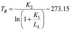 | (2) |
where:
TB = Satellite brightness temperature in the centigrade scale,
Lλ = Spectral radiance of TOA (Watts/(sq. m*srad*μm)),
K1 = Calibration constant 1,
K2 = Calibration constant 2.
According to Rai (2019), Equation (2) has specific values for coefficients K1 and K2 (see Table 1). So, the final expression, in order to estimate the Brightness Temperature, has the following form:
TB = (1321.0789 / ln((774.8853//TOA) + 1)) – 273.15
Table 1. Metadata from Landsat 8 Images
| Band 10 | |
|---|---|
| K1 | 774.8853 |
| K2 | 1321.0789 |
Source: adapted from: USGS, 2022c.
Normalized Difference Vegetation Index (NDVI): The following steps refer to the estimation of a very important index, known as the NDVI. As already stated, this index is based on the difference between the maximum reflectance in the NIR spectral region (which is a result of leaf cellular structure) and the maximum absorption of radiation in R (as an effect of chlorophyll pigments) (Tucker, 1979). Based on the above elements, the NDVI equation is formulated as follows and its numerical range is between [–1 to 1] (Jones and Vaughan, 2010):
 | (3) |
According to LANDSAT 8 measures and Table 2, the final expression of Equation (3) for further processing in the QGIS software uses the following equation: NDVI = Float (Band 5 – Band 4) / Float (Band 5 + Band 4)
| Bands | Wavelength (micrometres) | Resolution (meters) |
|---|---|---|
| Band 4 – Red | 0.64 – 0.67 | 30 |
| Band 5 – Near Infrared (NIR) | 0.85 – 0.88 | 30 |
| Band 6 – SWIR1 | 1.57 – 1.65 | 30 |
| Band 10 – Thermal Infrared (TIRS) 1 | 10.60 – 11.19 | 100 |
The proportion of Vegetation (Pv): Pv is known as the ratio of the vertical projection vegetation region on the ground to the total area of vegetation (Deardorff, 1978). Specifically, for the QGIS representation of this specific indicator, the formula obtained is the following (Carlson and Ripley, 1997):
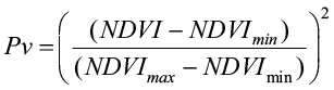 | (4) |
In QGIS software, the NDVI calculation is produced with a broad range of values. The solution in Equation (4) utilises the maximum and minimum values of the previous index.
Land Surface Emissivity (ε) is a significant element for the final equation and the calculation of Land Surface Temperature (LST). Land Surface Emissivity (LSE) uses the results of Equation (4) and by utilising the PV index it calculates the average emissivity of an element of the study area, based on the values of Equation (3) and the NDVI (Randhi et al., 2021):
| LSE = 0.004 * Pv + 0.986 | (5) |
where:
LSE = Land Surface Emissivity,
Pv = Proportion of Vegetation (%).
In this case, the 0.986 value is considered as a correction coefficient, while the 0.004 declares the standard deviation, considering a total of 49 soil spectrals from the ASTER spectral library (Sobrino et al., 2004).
Land Surface Temperature (LST): This is the final estimate of the entire aforementioned process, which combines all of the above results (Fig. 3). The variables BT, NDVI and LSE are the most significant factors for the LST calculation (Shah et al., 2018). This index includes a mix of vegetation and bare soil temperature and is defined as the radiative skin temperature of the land surface (Freitas et al., 2013; Kogan, 2001; Martins, J. P.; Wan et al., 1996).
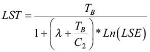 | (6) |
where:
LST = Land Surface Temperature (oC),
TB = Bright Temperature (BT) calculated from Equation (2),
λ = Constant value of 0.00115,
C2 = Constant value of 1.4388,
LSE = Land Surface Emissivity (LSE) calculated from Equation (5).
The final form of the equation is given below for the visualisation of the LST index in the QGIS software (Aryal et al., 2021):
LST = (TB / (1 + (0.00115 * TB / 1.4388) * Ln(LSE)))
Normalized Difference Build-up Index (NDBI): This variance is independent and does not belong to the LST calculation process. Its value ranges between –1 and 1, as in the case of the NDVI. The visualisation of this index reveals the points and/or locations in the urban fabric that are characterised by dense constructions and buildings (values that are close to 1) and areas with a low density of buildings (values that are close to –1) (Zha et al., 2003). Another noteworthy outcome is the expected strong negative correlation that is going to appear compared to the NDVI. Furthermore, the intense and continuous urban expansion increases the NDBI, and this is an important potential result of this index, in most LST-related studies (Chen et al., 2006). The last equation with regards to the LST index is the equation of the NDBI (Eq. (7)):
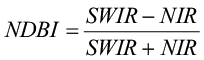 | (7) |
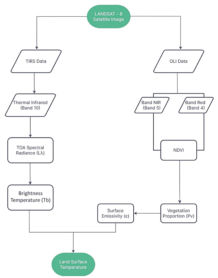
Fig. 3. Flowchart of the process for the Land Surface Temperature (LST) calculation
Source: own work.
Using the values from Table 2 the final expression of Equation (7) for further processing in the QGIS software uses the following equation:
NDBI = Float (Band 6 – Band 5) / Float (Band 6 + Band 5)
Normalized Difference Moisture Index (NDMI): It is used for vegetation water content determination. Its mathematical formula fits the case of the NDBI, but in this case the terms of the ratio are inverted (USGS, 2022b). Therefore, a significant expected outcome is the negative correlation between moisture and temperature. Moreover, the range value of this index fluctuates between -1 to 1 once again.
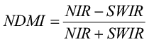 | (8) |
According to values in Table 2 the suitable form of Equation (8) using Bands 5 and 6 for the NDMI calculation (in the QGIS software) is the following:
NDMI = Float (Band 5 – Band 6) / Float (Band 5 + Band 6)
By utilising the interactive FloodMap Pro application, we aimed to accurately identify areas vulnerable to future sea level rise in Thessaloniki. We focused on areas that would be affected by sea level rise at the interval between 1 and 4 meters. For this particular interval there is no computational burden/cost as the FloodMap application provides the user with all the necessary information and results. Furthermore, the upper limit (4 meters) is considered as an extreme worst-case scenario for the study area. By following this method, we aimed to identify those (coastal) areas in the Municipality of Thessaloniki that should focus on climate change adaptation and specifically on enhancing their resilience to rising sea levels.
The third component of the Integrated Spatial Vulnerability Index (IntSpVI) is the Flood vulnerability index. In this context a number of flood vulnerability zones in the boundaries of the Municipality of Thessaloniki have been identified. To do so, the historical and significant floods were used as input data, were digitised through QGIS and were mapped in order to construct the vulnerable flood zones that should be considered in future urban reliance planning.
In order to identify areas the most vulnerable to climate change several data collection and processing methods were used. As a first step in data analysis, satellite images from the USGS (2022a), using the American Earth observation satellite Landsat 8, were used. More specifically, two satellite images were taken at specific intervals. The first one was taken on 12 Nov 2021 and represents the winter period under consideration with a cloud cover of less than 10%. The second satellite image was taken on 1 Aug 2021 as an indicative date for the summer period, with a similar percentage of cloud cover (Fig. 4a). These raster files were downloaded and analysed in the QGIS software in order to visualise important climatic and spectral indices, as well as geomorphological data related to elevation (Fig. 4b) and slope (Fig. 4c). In addition, by using the FloodMap Pro application it was possible to locate/identify the areas that could be affected by a future sea level rise. At the same time, historical flood data was collected for the study area.
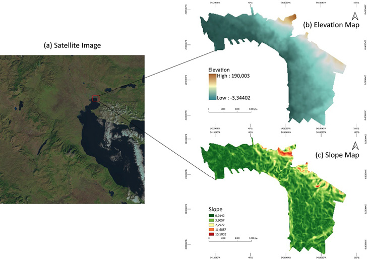
Fig. 4. Landsat – 8 Image of municipality location (a), elevation map of municipality (b) and slope map of municipality (c)
Source: own work.
The spatial analysis of spectral indices constitutes the most significant element for the estimation of the temperature variance in the study area. All the maps produced and presented below display a variance of the NDVI, NDBI, and NDMI indices between the winter and summer seasons. According to the selected satellite images, the NDVI has higher and more diverse values in summer (Fig. 5b) than in winter (Fig. 5a). This was actually an expected result due to the fact that during the warm months, the rise of temperature and summer heatwaves are likely to enhance flora growth. NDVI maps are useful for visualising the vegetation of the municipality, giving a general view of the situation, concerning vegetation cover and density that prevails within its boundaries. Green areas tend to be accumulated along a significant part of the municipality’s coastline, as well as at the western boundaries. It should be also noticed that a significant part of the study area, at the northern boundaries, is covered by forest. In addition, sparse concentrations of green areas are observed in the heart of the urban area. An interesting conclusion drawn from this analysis is that green spaces are cut off and discontinuous for the most of the study area surface, thus leading to the aggravation of high temperature problems.
The visualisation of the NDBI that follows reveals the intensity of the building stock on the surface of the municipality. The reason that NDBI is analysed both in winter (Fig. 5c) and summer (Fig. 5d) is to indirectly confirm the increase of the vegetation intensity during the summer months and, at the same time, to underline the absence of green spaces and the prevalence of built-up areas in the whole urban space. Finally, the NDMI examines the moisture levels of the surface of the study area. A noteworthy outcome is that during the summer period (Fig. 5f) NDMI values are significantly higher than during winter (Fig. 5e). This result confirms previous relevant studies, according to which the moisture levels are likely to rise on warmer days in coastal urban areas, like Thessaloniki.
Figure 6 depicts the outcome of the Land Surface Temperature (LST) model for the winter (Fig. 6a) and the summer period (Fig. 6b) in the study area. Both LST model’s results confirm high levels of land temperature in specific urban neighbourhoods. Namely, both maps indicate that the area near the port of Thessaloniki seems to be the area with the highest temperatures in the study area. As shown on the first map, the higher LST (located near the port) during winter is equal to 17.84oC (Fig. 6a), while during summer the higher LST value (also located near the port) rises to 42.05oC (Fig. 6b). Another part of the municipality affected by heatwaves is located at the mid-north of the city, in an overpopulated neighbourhood, which is characterised by an extremely high percentage of residential/build areas and completely sealed surfaces.

Fig. 5. Normalised Difference Vegetation Index (NDVI) – winter season (a), Normalised Difference Vegetation Index (NDVI) – summer season (b), Normalised Difference Built-up Index (NDBI) – winter season (c), Normalised Difference Built-up Index (NDBI) – summer season (d), Normalised Difference Moisture Index (NDMI) – winter season (e) and Normalised Difference Moisture Index (NDMI) – summer season (f)
Source: own work.
The higher discomfort within the municipality area, due to high temperatures, is partly due to inadequate vegetation cover (as depicted in the NDVI maps) and due to the dense building structures and sealed surfaces (as depicted in the NDBI maps). An equally important indicator that greatly influences the variations of the LST index are the variations of the moisture index (NDMI). It’s easily observable that the regions where the moisture levels are low, the temperatures levels increase (and vice versa). So, temperature variation was found, as expected, inversely proportional to the moisture variation.

Fig. 6. Land Surface Temperature (LST) – winter season (a) and Land Surface Temperature (LST) – summer season (b)
Source: own work.
In order to compare the land temperature between the highly urbanised study area with the surrounding rural areas, we estimated the LST for the summer period for an extended area (Fig. 7a), including a rural neighbourhood municipality (Municipality of Delta). As observed in the Corine Land Cover map (Fig. 7b), land uses in the Municipality of Delta (in the western part of the map) are typical rural, as the area is dominated by various agricultural and natural land cover types. LST differences between these rural areas and the study area (the city of Thessaloniki) are large, indicating the presence of an UHI effect.
A statistical analysis followed the visualisation of spectral indices and LST, with the aim to estimate the correlations between specific measurements/indices. This is considered as an important step in determining the factors that affect soil temperature and consequently the quality of citizens’ life (under the assumption that high/extreme summer temperatures are associated with social disutility).
The correlations were estimated by using the SPSS software (IBM-SPSS Statistics Software, Version 27), for both time periods examined (winter and summer). Regarding the winter period (Table 3) the LST index shows a positive correlation with the NDVI and NDBI and a negative correlation with the NDMI. Also, the relationship between temperature and building density is equally proportional, which is due to the large concentration of impermeable materials, pavements, and high-rise buildings, which accumulate heat and trap the sun’s rays due to low reflectivity. The moisture difference indicator is positively and highly correlated with vegetation levels and, therefore, its role is crucial for the formation of temperature levels in the urban space. The NDVI, in turn, shows a strong negative correlation with the NDBI. All the aforementioned correlations are statistically significant at the 5% level.
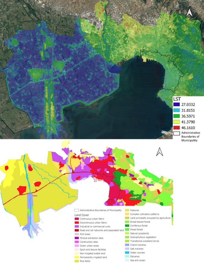
Fig. 7. (a) LST (summer season) comparison between urban and neighbouring rural areas (b) Corine land cover map
Source: own work.
The GeoDa software was then used to generate the scatterplot matrix presented in Fig. 8. The main purpose of this chart was to visualise all the bivariate correlations of Table 3. It is obvious that all bivariate correlations are statistically significant at the 1% level. However, it is also worth noticing that the LST index does not show a particularly strong correlation with the other spectral indices, for a number of reasons, which are going to be explained in the next section.
Table 3. Spectral indices and LST correlation for the winter period
| Correlations | |||||
|---|---|---|---|---|---|
| LST | NDVI | NDBI | NDMI | ||
| LST | Pearson Correlation | 1 | 0.168** | 0.094** | –0.094** |
| Sig. (2-tailed) | 0.000 | 0.008 | 0.008 | ||
| N | 805 | 805 | 805 | 805 | |
| NDVI | Pearson Correlation | 0.168** | 1 | –0.679** | 0.679** |
| Sig. (2-tailed) | 0.000 | 0.000 | 0.000 | ||
| N | 805 | 805 | 805 | 805 | |
| NDBI | Pearson Correlation | 0.094** | –0.679** | 1 | –1.000** |
| Sig. (2-tailed) | 0.008 | 0.000 | 0.000 | ||
| N | 805 | 805 | 805 | 805 | |
| NDMI | Pearson Correlation | –0.094** | 0.679** | –1.000** | 1 |
| Sig. (2-tailed) | 0.008 | 0.000 | 0.000 | ||
| N | 805 | 805 | 805 | 805 | |
| ** Correlation is significant at the 0.01 level (2-tailed) | |||||
Source: own work.
By analysing the bivariate correlations for the summer period, it is worth mentioning that the correlation between LST and NDVI is now negative and statistically significant (Table 4). The correlation between LST and NDMI continues to be negative but higher than during winter, while the same applies to the positive correlation between LST and NDBI. During the summer months, the vegetation index shows a higher (and still negative) correlation value (as compared to winter) with the building stock (NDBI).
The same conclusions as when it comes to the winter period (Fig. 8) can be drawn from Figure 9 (summer period). Namely, the LST index has medium to low correlations with all other indices, which is partly attributed to the small number of observations (N = 805) and the homogeneity in land uses and (micro)climate conditions. The correlations coefficients (as compared to Fig. 8) are increased between the indices NDVI, NDBI and NDMI, while the absolute negative correlation between NDBI and NDMI is almost identical.
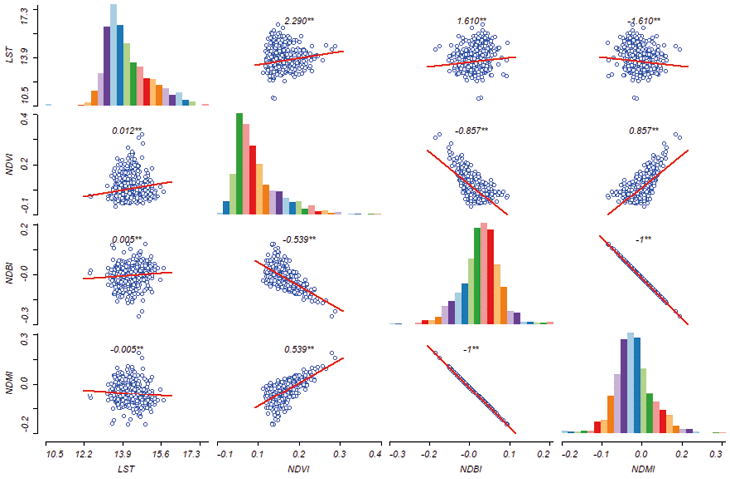
Fig. 8. Scatterplot matrix for the winter period
Source: own work.
Table 4. Spectral indices and LST correlation for the summer period
| Correlations | |||||
|---|---|---|---|---|---|
| LST | NDVI | NDBI | NDMI | ||
| LST | Pearson Correlation | 1 | –0.142** | 0.238** | –0.226** |
| Sig. (2-tailed) | 0.000 | 0.000 | <0.001 | ||
| N | 805 | 805 | 805 | 805 | |
| NDVI | Pearson Correlation | –0.142** | 1 | –0.756** | 0.752** |
| Sig. (2-tailed) | 0.000 | 0.000 | <0.001 | ||
| N | 805 | 805 | 805 | 805 | |
| NDBI | Pearson Correlation | 0.238** | –0.756** | 1 | –1.000** |
| Sig. (2-tailed) | 0.000 | 0.000 | |||
| N | 805 | 805 | 805 | 805 | |
| NDMI | Pearson Correlation | –0.226** | 0.752** | –1.000** | 1 |
| Sig. (2-tailed) | <0.001 | <0.001 | 0.000 | ||
| N | 805 | 805 | 805 | 805 | |
| ** Correlation is significant at the 0.01 level (2-tailed) | |||||
Source: own work.
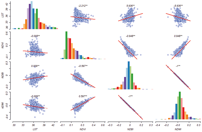
Fig. 9. Scatterplot matrix for the summer period
Source: own work.
The positive correlations found between temperature and vegetation during winter are consistent with the results of previous studies (Kaufmann et al., 2003; Sun and Kafatos, 2007). Concerning the summer period, the negative correlations between LST and NDVI are once again similar to the results of relevant literature (Nemani et al., 1993; Gorgani et al., 2013). However, in contrast to the findings of Malik et al. (2019) who estimated a powerful correlation between LST and NDBI, in our study we only found a weak yet still statistically significant correlation. A possible reason for this is the fact that the entire study area is quite homogenous in terms of land-uses and (urban) built-up environment.
Furthermore, our results confirm the findings of Li et al. (2017), who revealed a stronger correlation between the LST index and NDMI than between temperature (LST) and vegetation (NDVI). Therefore, our study proves the conclusion highlighted by Li et al. (2017), about the greater importance of the moisture difference index (NDMI) than the vegetation index (NDVI) in explaining the spatial variation of surface temperature.
The lack of urban green areas and the extended waterfront (coastline) are the most important reasons for the presence of an extensive area of potentially high flood risk. Coastal urban communities A, B, and E, but also the inland community D (Fig. 10) are considered quite vulnerable to urban flooding, which is mainly associated with flash flooding. Some geomorphological and physical factors that increase the flood risk/vulnerability are low altitude (Fig. 4b) and slope (Fig. 4c), as well as the strong presence of (subterranean) streams mainly in communities A, D, and E. Based on the historical and important recorded rainfalls and floods, the area where communities A and E overlap is the most vulnerable to floods, due to its low altitude, and the presence of many streams prone to flash flooding.
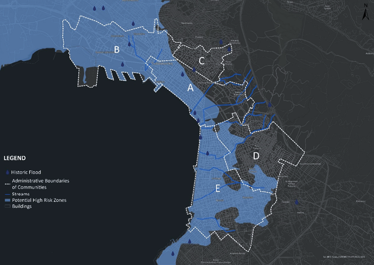
Fig. 10. Potential high-risk zone in floods
Source: own work.
One of the most important reasons for the enhancement of climate change mitigation policies is the melting of ice and the rising sea level. According to scientific research, if humanity follows a sustainable path, the sea level could rise by 30 cm by 2100. In the pessimistic (non-sustainable) scenario the increase of the sea level could reach 2.5 meters (IPCC, 2019). The FloodMap Pro application digitises the coastal areas that are going to be affected by the sea level. The central port area in Community B (Fig. 11b) is going to face the greatest consequences in the absence of any risk/climate resilience planning. In addition, the coastal zone in the historical centre of the city, in Community A (Fig. 11a), may also face similar consequences, however, in a much smaller and less structured area. Significantly, a quite densely populated area with high real estate values in Community E (Fig. 11c) is also found to be vulnerable to long-term sea level rise.
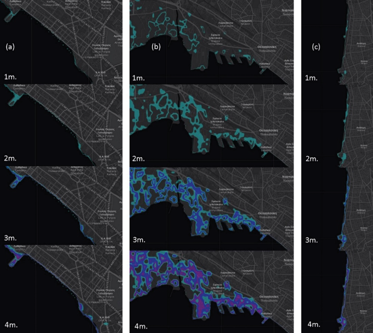
Fig. 11. Four scenarios of sea level rise in the coastline of Community B (a), Community A (b), and Community E (c)
Source: own work adapted from FloodMap Pro.
Moran’s I, involving Global (Moran, 1950) and Local (Anselin, 1995) Moran’s I, is a commonly used indicator of spatial autocorrelation. In this study, the Local Moran’s I index and the GeoDa software were used to delimit areas affected by high temperatures, by implementing spatial autocorrelation analyses. Specifically, a Lisa (Local Indicators of Spatial Association) analysis was used, according to five classes according to the map’s legend (Fig. 12). A high positive local Moran’s I value indicates a location which has similarly high or low values as its neighbours. These locations are ‘spatial cluster’, which may be either high-high clusters (high values in a high-value neighbourhood) or low-low clusters (low value in a low-value neighbourhood) (Zhang et al., 2008), while negative local Moran’s I values (low-high or high-low) indicate potential spatial outliers (i.e., locations that are different in terms of their values from their neighbours) (Lalor and Zhang, 2001).
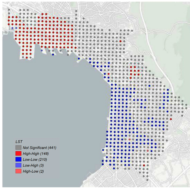
Fig. 12. Spatial autocorrelation of high temperature
Source: own work.
In Fig. 12, the colour classes are attributed to statistically significant clusters/areas which experience greater (red dots) or lower (blue dots) discomfort (as compared to the rest of the urban area) due to high summer temperatures. A large part of the second community and the port area seems to be the most affected, having a high-high positive autocorrelation, while a significant part of communities D and E and part of the historic city centre (community A) close to the waterfront experience lower temperature during the summer period.
The final aim of this paper is to create an integrated spatial vulnerability index. Therefore, the vulnerable regions presented in Figures 6, 10, and 11 have been combined to create a single vulnerability map (Fig. 13). Figure 13 represents all the areas vulnerable to extreme weather phenomena (temperature and floods). In all the red-coloured areas, where temperatures exceed normal levels, the absence of green and open spaces is obvious. These areas are also characterised by dense building structures and impermeable surfaces. Therefore, these areas were found to possess high NDBI and low NDVI and NDMI values. At the same time, the potential zone of high flood risk extends over a very large area due to the low altitude, but also to the small slopes. Also, the total absence of green infrastructure leads to an inability to absorb rainwater (as nature-based solutions), while the dense urban development enhances the risks of urban (flash) flooding. Finally, the sea level rise is going to affect only some small/local coastal (though with significant landmarks) high real estate values and important economic activities.
In this study, a model was developed through satellite imageries for the estimation of the LST index and other important spectral indicators, which are likely to affect and being affected by temperature spatial variation. With the help of Landsat-8 satellite imagery, our model mapped as accurately as possible the ground temperature and the vegetation spectrum, the intensity of the building stock/structures, and the moisture difference at a spatial resolution of 30 to 100 meters. Based on the statistical analysis developed, the selected indicators revealed a variety of correlations and interactions among them.
Specifically, the LST index and NDVI showed a positive correlation in winter and a negative correlation in summer, while the correlation of the former with NDBI was positive in both cases (periods). All binomial correlations with the LST were found statistically significant but not very strong, mainly due to the relatively small number of observations and the homogeneity of land uses (spatial uniformity). In addition, the correlations between vegetation levels (NDVI) and structure levels (NDBI) as well as the moisture differences (NDMI) are quite satisfactory in both periods.
A few limitations of our study need to be acknowledged. Firstly, a possible limitation of this study is that we did not have time-series data for analysis but only data for a specific year (2021). Furthermore, the use of NDVI as a proxy for vegetation cover may cause some problems due to the fact that it represents an aggregate measure of green vegetation and, therefore, it is not always a perfect proxy for all types of urban vegetation, especially with reference to their cooling potential (e.g., trees also contributing to local cooling by providing shade). By using the LST it was not possible to consider air temperature, so we could not estimate the effect on ambient air temperature of such factors as the building side walls and/or the ground below tree canopy. Another limitation was that we did not account for population exposure on climate related hazards. The populations at risk and their socio-economic characteristics could provide a more complete picture.

Fig. 13. Regions vulnerable to high temperatures and floods
Source: own work.
Most of the areas that experience higher temperatures in summer have the same characteristics: limited or total lack of vegetation, absence of free open spaces, and a high density of buildings. Furthermore, as the final aim of this study was to provide an integrated spatial vulnerability index to climate change, we also examined the urban areas that are prone to (flash) flooding and sea level rise. Once again, the absence of green spaces, the high building density, and the dominance of sealed/impermeable surfaces are the main drivers for increasing flood-related risks. The final vulnerability map, which incorporates all the above-mentioned climate-related risks, depicts that the city of Thessaloniki is not highly resistant to climate change as many areas/neighbourhoods are exposed to one or more risk factors. Therefore, future urban planning should in general focus on climate change adaptability by ensuring long-term investments in (urban) green infrastructure and nature-based solutions. Furthermore, the application of the IntSpVi also provides useful information to the competent authorities for identifying areas that are more exposed to extreme temperatures and intense flood events. Thus, it would be possible to prioritise those neighbourhoods/areas where specific future planning interventions (for climate change adaptation) should occur.
A very important element of the urban structure that may help to mitigate the problem of the UHI and urban floods (by using a nature-based solution) is green infrastructure. The planning of urban greenery has been the major tool applied worldwide to mitigate the UHI (Dos Santos et al., 2017), which has also several co-benefits (e.g., supporting urban biodiversity, improving air quality, carbon sequestration, etc.). Unfortunately, as already stated, Thessaloniki is a typical compact city facing a lack of urban green spaces, which are highly fragmented, and their size is usually small (only 30% of them are larger than 0.5 ha). Therefore, local authorities should incorporate green infrastructure into policies and practices where possible to reduce the overall heat stress vulnerability and to provide thermal comfort. In other words, it is necessary to explore the possibility of redesigning and expanding the existing green infrastructure (Kazak, 2018). The effort to unify the fragmented and discontinuous urban green spaces through green corridors and pocket parks will further contribute to the reduction of both thermal stress and flood risks.
The results of the IntSpVi can also be utilised by the insurance sector. Namely, areas with higher vulnerability values prone to more than one climate-related hazard may affect future insurance rates, which incorporate/reflect the level of associated risk. Land values may also be affected in the long term. So, houseowners and landowners in areas with higher vulnerability may have an increased interest in various adaptation (e.g., nature-based) solutions that could reduce future risks and to minimise any negative impacts on their real-estate values. As a consequence, spatial information provision on climate-related vulnerability may force communities and stakeholders to play a role in building urban resilience by exerting pressure on the local authorities to reduce the future impacts/risks of climate change.
ALEXANDER, C. (2020), ‘Normalised difference spectral indices and urban land cover as indicators of land surface temperature (LST)’, International Journal of Applied Earth Observation and Geoinformation, 86, 102013. https://doi.org/10.1016/j.jag.2019.102013
ANDERSON, M. C., NORMAN, J. M., KUSTAS, W. P., HOUBORG, R., STARKS, P. J. and AGAM, N. (2008), ‘A thermal-based remote sensing technique for routine mapping of land-surface carbon, water, and energy fluxes from field to regional scales’, Remote Sensing of Environment, 112, pp. 4227–4241. https://doi.org/10.1016/j.rse.2008.07.009
ANSELIN, L. (1995), ‘Local indicators of spatial association—LISA’, Geographical Analysis, 27 (2), pp. 93–115.
ANSELIN, L., SYABRI, I. and KHO, Y. (2010), GeoDa: an introduction to spatial data analysis. In Handbook of applied spatial analysis, Berlin, Heidelberg: Springer, pp. 73–89.
ARYAL, A., SHAKYA, B., MAHARJAN, M., TALCHABHADEL, R. and THAPA, B. (2021), Evaluation of the Land Surface Temperature using Satellite Images in Kathmandu Valley, 1, pp. 1–10.
ARTIS, D. A. and CARNAHAN, W. H. (1982), ‘Survey of emissivity variability in thermography of urban areas’, Remote Sensing of Environment, 12, pp. 313–329. https://doi.org/10.1016/0034-4257(82)90043-8
ASHRAF, M. and NAWAZ, R. (2015), ‘A Comparison of Change Detection Analyses Using Different Band Algebras for Baraila Wetland with Nasa’s Multi-Temporal Landsat Dataset’, JGIS, 07, pp. 1–19. https://doi.org/10.4236/jgis.2015.71001
BOSELLO, F. and DE CIAN, E. (2014), ‘Climate change, sea level rise, and coastal disasters. A review of modeling practices’, Energy Economics, 46, pp. 593–605.
BRUNSELL, N. A. and GILLIES, R. R. (2003), ‘Length Scale Analysis of Surface Energy Fluxes Derived from Remote Sensing’, Journal of Hydrometeorology, 4, pp. 1212–1219. https://doi.org/10.1175/1525-7541(2003)004<1212:LSAOSE>2.0.CO;2
BUCHHOLZ, S., KOSSMANN, M. and ROOS, M. (2016), ‘INKAS–a guidance tool to assess the impact of adaptation measures against urban heat’, Meteorologische Zeitschrift, 25 (3), pp. 281–289.
BUYANTUYEV, A. and WU, J. (2010), ‘Urban heat islands and landscape heterogeneity: linking spatiotemporal variations in surface temperatures to land-cover and socioeconomic patterns’, Landscape Ecol, 25, pp. 17–33. https://doi.org/10.1007/s10980-009-9402-4
CARLSON, T. N. and RIPLEY, D. A. (1997), ‘On the relation between NDVI, fractional vegetation cover, and leaf area index’, Remote Sensing of Environment, 62, pp. 241–252. https://doi.org/10.1016/S0034-4257(97)00104-1
CHANGNON, S. A., KUNKEL, K. E. and REINKE, B. C. (1996), ‘Impacts and responses to the 1995 heat wave: A call to action’, Bulletin of the American Meteorological Society, 77, pp. 1497–1505.
CHEN, X.-L., ZHAO, H.-M., LI, P.-X. and YIN, Z.-Y. (2006), ‘Remote sensing image-based analysis of the relationship between urban heat island and land use/cover changes’, Remote Sensing of Environment, Thermal Remote Sensing of Urban Areas, 104, pp. 133–146. https://doi.org/10.1016/j.rse.2005.11.016
CHEN, L., LI, M., HUANG, F. and XU, S. (2013), ‘Relationships of LST to NDBI and NDVI in Wuhan City based on Landsat ETM+ image’, [in:] 2013 6th International Congress on Image and Signal Processing (CISP), presented at the 2013 6th International Congress on Image and Signal Processing (CISP), pp. 840–845. https://doi.org/10.1109/CISP.2013.6745282
DEARDORFF, J. W. (1978), ‘Efficient prediction of ground surface temperature and moisture, with inclusion of a layer of vegetation’, Journal of Geophysical Research: Oceans, 83, pp. 1889–1903. https://doi.org/10.1029/JC083iC04p01889
DEDEKORKUT-HOWES, A., TORABI, E. and HOWES, M. (2020), ‘When the tide gets high: A review of adaptive responses to sea level rise and coastal flooding’, Journal of Environmental Planning and Management, 63 (12), pp. 2102–2143.
DONG, W., LIU, Z., ZHANG, L., TANG, Q., LIAO, H. and LI, X. (2014), ‘Assessing heat health risk for sustainability in Beijing’s urban heat island’, Sustainability, 6, pp. 7334–7357.
DOS SANTOS, A. R., DE OLIVEIRA, F. S., DA SILVA, A. G., GLERIANI, J. M., GONÇALVES, W., MOREIRA, G. L., SILVA, F. G., BRANCO, E. R. F., MOURA, M. M., DA SILVA, R. G. and JUVANHOL, R. S. (2017), ‘Spatial and temporal distribution of urban heat islands’, Science of the Total Environment, 605, pp. 946–956.
FREITAS, S. C., TRIGO, I., MACEDO, J., BARROSO, C., SILVA, R. and PERDIGAO, R. (2013), ‘Land Surface Temperature from multiple geostationary satellites’, International Journal of Remote Sensing, 34, pp. 3051–3068.
Flood Map: Elevation Map, Sea Level Rise Map, n.d. URL https://www.floodmap.net/ [accessed on: 19.08.2022].
GARZILLO, C. and ULRICH, P. (2015), Annex to MS94: Compilation of case study reports A compendium of case study reports from 40 cities in 14 European countries, 94. WWWforEurope Working Paper.
GEMENETZI, G. (2017), ‘Thessaloniki: The changing geography of the city and the role of spatial planning’, Cities, 64, pp. 88–97. https://doi.org/10.1016/j.cities.2016.10.007
GISGEOGRAPHY (2019), Landsat 8 Bands and Band Combinations. GIS Geography. URL https://gisgeography.com/landsat-8-bands-combinations/ [accessed on: 21.02.2022].
GORGANI, S., PANAHI, M. and REZAIE, F. (2013), The Relationship between NDVI and LST in the urban area of Mashhad, Iran.
HAINES, A., KOVATS, R. S., CAMPBELL-LENDRUM, D. and CORVALAN, C. (2006), ‘Climate change and human health: Impacts, vulnerability and public health’, Public Health, 120, pp. 585–596. https://doi.org/10.1016/j.puhe.2006.01.002
IPCC, 2014. CLIMATE CHANGE (2014), ‘Synthesis report’, [in:] Core Writing Team, R. K. Pachauri and L. A. Meyer (eds.), Contribution of Working Groups I, II and III to the Fifth Assessment Report of the Intergovernmental Panel on Climate Change. IPCC: Geneva, Switzerland, pp. 1–112. https://doi.org/10.1017/CBO9781107415324
IPCC (2018), Special Report: Global Warming of 1.5 ºC, Incheon: Intergovernmental Panel on Climate Change.
IPCC (2019), ‘Summary for Policymakers’, [in:] IPCC Special Report on the Ocean and Cryosphere in a Changing Climate [H.-O. Pörtner, D. C. Roberts, V. Masson-Delmotte, P. Zhai, M. Tignor, E. Poloczanska, K. Mintenbeck, M. Nicolai, A. Okem, J. Petzold, B. Rama, N. Weyer (eds.)]. Forthcoming. https://www.ipcc.ch/srocc/chapter/summary-for-policymakers/ [accessed on: 21.02.2022].
JAVED, M., KRISHNANAND, S. H., NAGABHUSHAN, P. and CHAUDHURI, B. B. (2016), ‘Visualizing CCITT Group 3 and Group 4 TIFF Documents and Transforming to Run-Length Compressed Format Enabling Direct Processing in Compressed Domain’, Procedia Computer Science, International Conference on Computational Modelling and Security, 85, pp. 213–221. https://doi.org/10.1016/j.procs.2016.05.214
JONES, H. G. and VAUGHAN, R. A. (2010), Remote Sensing of Vegetation: Principles, Techniques, and Applications, Oxford, New York: Oxford University Press.
JU, Y., LINDBERGH, S., HE, Y. and RADKE, J. D. (2019), ‘Climate-related uncertainties in urban exposure to sea level rise and storm surge flooding: a multi-temporal and multi-scenario analysis’, Cities, 92, pp. 230–246.
KANTZIOURA, A., KOSMOPOULOS, P. and ZORAS, S. (2012), ‘Urban surface temperature and microclimate measurements in Thessaloniki’, Energy and Buildings, 44, pp. 63–72. https://doi.org/10.1016/j.enbuild.2011.10.019
KAUFMANN, R. K., ZHOU, L., MYNENI, R. B., TUCKER, C. J., SLAYBACK, D., SHABANOV, N. V. and PINZON, J. (2003), ‘The effect of vegetation on surface temperature: A statistical analysis of NDVI and climate data’, Geophysical Research Letters, 30. https://doi.org/10.1029/2003GL018251
KAZAK, J. K. (2018), ‘The use of a decision support system for sustainable urbanization and thermal comfort in adaptation to climate change actions – The case of the Wrocław larger urban zone (Poland)’, Sustainability, 10 (4), 1083, pp. 1-15.
KLEEREKOPER, L., van ESCH, M. and SALCEDO, T. B. (2012), ‘How to make a city climate-proof, addressing the urban heat island effect’, Resources, Conservation and Recycling, Climate Proofing Cities, 64, pp. 30–38. https://doi.org/10.1016/j.resconrec.2011.06.004
KIM, H. H. (1992), ‘Urban heat island’, International Journal of Remote Sensing, 13 (12), pp. 319– 336.
KING, A. D. and KAROLY, D. J. (2017), ‘Climate extremes in Europe at 1.5 and 2 degrees of global warming. Environ’, Res. Lett., 12, 114031. https://doi.org/10.1088/1748-9326/aa8e2c
KOGAN, F. (2001), ‘Operational Space Technology for Global Vegetation Assessment’, Bulletin American Meteorological Society, pp. 1949–1964.
KONOPACKI, S. and AKBARI, H. (2002), Energy savings for heat island reduction strategies in Chicago and Houston (including updates for Baton Rouge, Sacramento, and Salt Lake City), Draft Final Report, LBNL-49638, University of California, Berkeley.
KUMARI, P., GARG, V., KUMAR, R. and KUMAR, K. (2021), ‘Impact of urban heat island formation on energy consumption in Delhi’, Urban Climate, 36, 100763.
LALOR, G. C. and ZHANG, C. (2001), ‘Multivariate outlier detection and remediation in geochemical databases’, Science of the total environment, 281 (1–3), pp. 99–109.
LATIF, M. S. (2014), Land Surface Temperature Retrival of Landsat-8 Data Using Split Window Algorithm – A Case Study of Ranchi District.
LATINOPOULOS, D., MALLIOS, Z. and LATINOPOULOS, P. (2016), ‘Valuing the benefits of an urban park project: A contingent valuation study in Thessaloniki, Greece’, Land Use Policy, 55, pp. 130–141.
LI, B. H. W. (2017), ‘Comparative study on the correlations between NDVI, NDMI and LST’, Advances in Geographical Sciences, 36, pp. 585–596. https://doi.org/10.18306/dlkxjz.2017.05.006
MALIK, M. S., SHUKLA, J. P. and MISHRA, S. (2019), ‘Relationship of LST, NDBI and NDVI using Landsat-8 data in Kandaihimmat Watershed, Hoshangabad, India’, Indian Journal of Geo-Marine Sciences, 48 (01), pp. 25–31.
MARINO, F. (2017), ‘Top of Atmosphere Reflectance on Sentinel 3’, Earth Starts Beating. https://www.earthstartsbeating.com/2017/04/27/top-of-atmosphere-reflectance-on-sentinel-3/ [accessed on: 21.02.2022].
MARTINS, J. P. (1999), The Hourly Land Surface Temperature from the Copernicus Global Land Service – Part 1: the updated algorithm with inclusion of vegetation dynamics and of Indian Ocean Data Coverage mission.
MATSA, M. and MUPEPI, O. (2022), ‘Flood risk and damage analysis in urban areas of Zimbabwe. A case of 2020/21 rain season floods in the city of Gweru’, International Journal of Disaster Risk Reduction, 67, 102638. https://doi.org/10.1016/j.ijdrr.2021.102638
MEMON, R. A., LEUNG, D. Y. C. and LIU, C. H. (2009), ‘An investigation of urban heat island intensity (UHII) as an indicator of urban heating’, Atmospheric Research, 94, pp. 491–500.
MORAN, P. A. P. (1950), ‘Notes on continuous stochastic phenomena’, Biometrika, 37 (1–2), pp. 17–23.
MUSHORE, T. D., MUTANGA, O. and ODINDI, J. (2022), ‘Estimating urban LST using multiple remotely sensed spectral indices and elevation retrievals’, Sustainable Cities and Society, 78, 103623. https://doi.org/10.1016/j.scs.2021.103623
NEMANI, R., PIERCE, L., RUNNING, S. and GOWARD, S. (1993). ‘Developing Satellite-derived Estimates of Surface Moisture Status’, Journal of Applied Meteorology and Climatology, 32, pp. 548–557. https://doi.org/10.1175/1520-0450(1993)032<0548:DSDEOS>2.0.CO;2
OKE, T. R. (1982), ‘The energetic basis of the urban heat island’, Quarterly Journal of the Royal Meteorological Society, 108, pp. 1–24. https://doi.org/10.1002/qj.49710845502
PITIDIS, V., TAPETE, D., COAFFEE, J., KAPETAS, L. and PORTO DE ALBUQUERQUE, J. (2018), ‘Understanding the implementation challenges of urban resilience policies: Investigating the influence of urban geological risk in Thessaloniki, Greece’, Sustainability, 10 (10), 3573.
PURVIS, M. J., BATES, P. D. and HAYES, C. M. (2008), ‘A probabilistic methodology to estimate future coastal flood risk due to sea level rise’, Coastal Engineering, 55 (12), pp. 1062–1073.
QGIS DEVELOPMENT TEAM (2019), QGIS Geographic Information System (3.6). Open Source Geospatial Foundation Project. https://www.qgis.org
QIAO, Z., TIAN, G., ZHANG, L., and XU, X. (2014), ‘Influences of urban expansion on urban heat island in Beijing during 1989–2010’, Advances in Meteorology, 2014, pp. 1–11.
RAI, R. (2019), Assessment of LST Variation in Kathmandu, Nepal. ArcGIS StoryMaps. https://storymaps.arcgis.com/stories/a70d27a801bf4972a005e03cb004e068 [accessed on: 21.02.2022]
RANDHI, U. D., SWARAJ, J., KUMAR, K. S. and PATRUDU, T. B. (2021), Sensible heat flux characterization using satellite remote sensing techniques, 6.
RIZWAN, A. M., DENNIS, L. Y. C. and LIU, C. (2008), ‘A review on the generation, determination and mitigation of Urban Heat Island’, Journal of Environmental Sciences, 20, pp. 120–128. https://doi.org/10.1016/S1001-0742(08)60019-4
ROY, D. P., KOVALSKYY, V., ZHANG, H. K., VERMOTE, E. F., YAN, L., KUMAR, S. S. and EGOROV, A. (2016), ‘Characterization of Landsat-7 to Landsat-8 reflective wavelength and normalized difference vegetation index continuity’, Remote Sensing of Environment, Landsat 8 Science Results, 185, pp. 57–70. https://doi.org/10.1016/j.rse.2015.12.024
SANTAMOURIS, M., CARTALIS, C., SYNNEFA, A. and KOLOKOTSA, D. (2015), ‘On the impact of urban heat island and global warming on the power demand and electricity consumption of buildings-a review’, Energy and Buildings, 98, pp. 119–124.
SEDAGHAT, A. and SHARIF, M. (2022), ‘Mitigation of the impacts of heat islands on energy consumption in buildings: A case study of the city of Tehran, Iran’, Sustainable Cities and Society, 76, 103435. https://doi.org/10.1016/j.scs.2021.103435
SHAH, S., SHRESTHA, R., TIMILSINA, P. and THAPA, M. (2018), Satellite Imagery Based Observation of Land Surface Temperature of Kathmandu Valley 7, 8.
SHARMA, A., WASKO, C. and LETTENMAIER, D. P. (2018), ‘If precipitation extremes are increasing, why aren’t floods?’, Water Resources Research, 54, pp. 8545– 8551.
SMITH, T. M., REYNOLDS, R. W., PETERSON, T. C. and LAWRIMORE, J. (2008), ‘Improvements to NOAA’s Historical Merged Land–Ocean Surface Temperature Analysis (1880–2006)’, Journal of Climate, 21, pp. 2283–2296. https://doi.org/10.1175/2007JCLI2100.1
SOBRINO, J. A., JIMÉNEZ-MUÑOZ, J. C. and PAOLINI, L. (2004), ‘Land surface temperature retrieval from LANDSAT TM 5’, Remote Sensing of Environment, 90, pp. 434–440. https://doi.org/10.1016/j.rse.2004.02.003
STAMOU, A., MANIKA, S. and PATIAS, P. (2013), ‘Estimation of land surface temperature and urban patterns relationship for urban heat island studies’, International Conference on Changing Cities: Spatial, morphological, formal & socio-economic dimensions, 18 to 21 June 2013, Skiathos island, pp. 2007–2013.
STATHOPOULOU, M., CARTALIS, C. and KERAMITSOGLOU, I. (2004), ‘Mapping micro-urban heat islands using NOAA/AVHRR images and CORINE Land Cover: an application to coastal cities of Greece’, International Journal of Remote Sensing, 25, pp. 2301–2316. https://doi.org/10.1080/01431160310001618725
STATHOPOULOU, M. and CARTALIS, C. (2007), ‘Daytime urban heat islands from Landsat ETM+ and Corine land cover data: An application to major cities in Greece’, Solar Energy, 81, pp. 358–368. https://doi.org/10.1016/j.solener.2006.06.014
SU, W., ZHANG, Y., YANG, Y. and YE, G. (2014), ‘Examining the impact of greenspace patterns on land surface temperature by coupling LiDAR data with a CFD model’, Sustainability, 6 (10), pp. 6799–6814.
SUN, D. and KAFATOS, M. (2007), ‘Note on the NDVI-LST relationship and the use of temperature-related drought indices over North America’, Geophysical Research Letters, 34. https://doi.org/10.1029/2007GL031485
TUCKER, C. J. (1979), ‘Red and photographic infrared linear combinations for monitoring vegetation’, Remote Sensing of Environment, 8, pp. 127–150. https://doi.org/10.1016/0034-4257(79)90013-0
TUCKER, C. J., PINZON, J. E., BROWN, M. E., SLAYBACK, D. A., PAK, E. W., MAHONEY, R., VERMOTE, E. F. and EL SALEOUS, N. (2005), ‘An extended AVHRR 8‐km NDVI dataset compatible with MODIS and SPOT vegetation NDVI data’, International Journal of Remote Sensing, 26, pp. 4485–4498. https://doi.org/10.1080/01431160500168686
USGS (2022a), Using the USGS Landsat Level-1 Data Product, U.S. Geological Survey, n.d. https://www.usgs.gov/landsat-missions/using-usgs-landsat-level-1-data-product [accessed on: 18.02.2022].
USGS (2022b), Normalized Difference Moisture Index, U.S. Geological Survey, n.d. https://www.usgs.gov/landsat-missions/normalized-difference-moisture-index [accessed on: 01.03.2022].
USGS (2022c), What are the band designations for the Landsat satellites?, U.S. Geological Survey, n.d. https://www.usgs.gov/faqs/what-are-band-designations-landsat-satellites [accessed on: 01.03.2022].
VOOGT, J. A. and OKE, T. R. (2003), ‘Thermal remote sensing of urban climates’, Remote sensing of environment, 86 (3), pp. 370–384.
WAN, Z., DOZIER, J. and DOZIER, J. (1996), ‘A generalized split-window algorithm for retrieving land-surface temperature from space’, IEEE Transactions on Geoscience and Remote Sensing, 34, pp. 892–905. https://doi.org/10.1109/36.508406
WWF GREECE, Climate change impacts in Greece in the near future, Athens, September 2009.
XIA, J., FALCONER, R. A., LIN, B. and TAN, G. (2011), ‘Modelling flash flood risk in urban areas’, [in:] Proceedings of the Institution of Civil Engineers-Water Management, 164 (6), pp. 267–282, Thomas Telford Ltd.
YIANNAKOU, A. and SALATA, K. D. (2017), ‘Adaptation to climate change through spatial planning in compact urban areas: a case study in the city of Thessaloniki’, Sustainability, 9 (2), p. 271.
ZHA, Y., GAO, J. and NI, S. (2003), ‘Use of normalized difference built-up index in automatically mapping urban areas from TM imagery’, International Journal of Remote Sensing, 24, pp. 583–594. https://doi.org/10.1080/01431160304987
ZHANG, C., LUO, L., XU, W. and LEDWITH, V. (2008), ‘Use of local Moran’s I and GIS to identify pollution hotspots of Pb in urban soils of Galway, Ireland’, Science of the Total Environment, 398 (1–3), pp. 212–221.
ZHOU, D., ZHANG, L., HAO, L. SUN, G., LIU, Y. and ZHU, C. (2016), ‘Spatiotemporal trends of urban heat island effect along the urban development intensity gradient in China’, Science of the Total Environment, 544, pp. 617–626.